Chapter 6: Wormhole’s Appearances and Properties

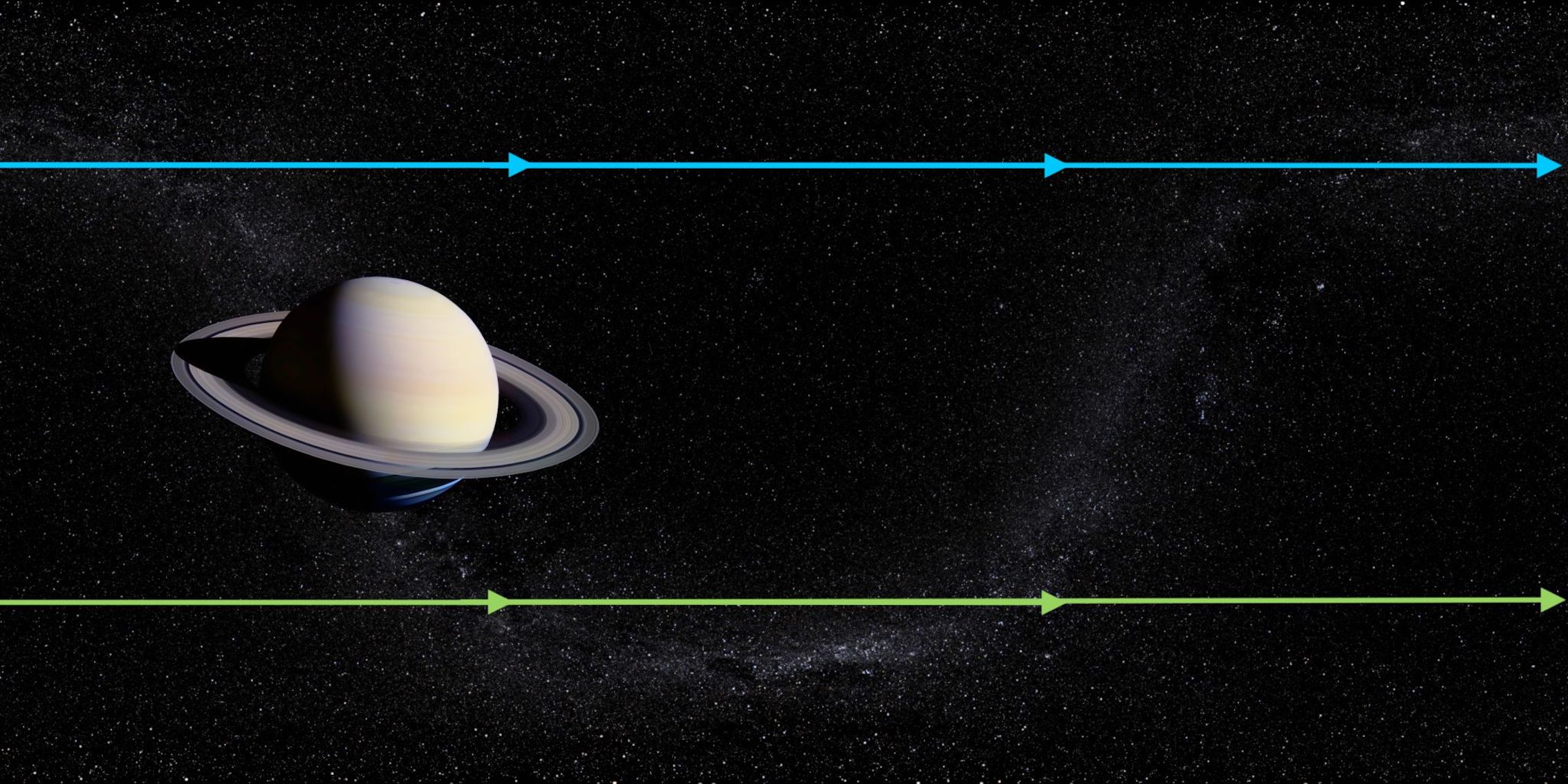
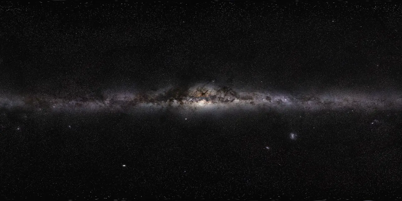
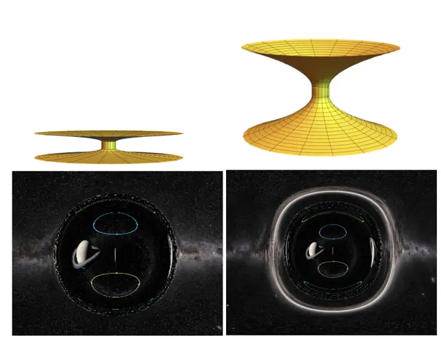
Using the algorithm and code derived in the last chapter, we can start producing images of wormholes with varying parameters. The two images in Figure 6.1 will be used as the celestial spheres on either side of the wormhole. The first image on the left is of Saturn that will be placed on the upper celestial sphere, which has been taken from the DN team’s website, ^[10]. On this image we have added two lines with arrows on them to understand the way the images are being distorted. The second image on the right is of Figure 6.1 of the Milky Way that was also used as the celestial sphere for the Schwarzschild black hole, which will be placed on the lower celestial sphere of our wormhole. This image is taken from the panorama taken by Brunier, ^[9].

Addition of these parameter is so that we can allow light to travel on numerous paths along the wormhole’s manifold. This allows us to gain a better understanding of how the light curves around the wormhole, and which rays make it to the camera. Instead of analysing images of wormholes with arbitrary parameters, we will keep some of the parameters constant, while varying one parameter at a time to compare the results, starting with the wormhole’s length.

6.1 Altering the Wormhole’s Length

Setting the parameters of the wormhole to $(\rho, \mathcal{W}, a)=(4, 0.2,a)$ where $a$ takes the values of $(0.02, 2, 20)$ produces the embedded diagrams of these wormholes respectively in the top images of Figure 6.2. Placing the images in Figure 6.1 on the celestial spheres and setting the camera’s local sky at coordinates $(l_c,\theta_c, \phi_c)=(\rho/2 +a, \pi/2, 0)$ produces the images that are on the bottom of these embedded diagrams that represents the images of these wormholes from the camera’s perspective. The lensing width has been set at a value of $0.05\rho$, so that the parameters have been kept constant, and the camera’s location has been set at a fixed distance of $\rho/2$ from the wormholes mouth so that the image comparison can be directly related to the wormholes length.

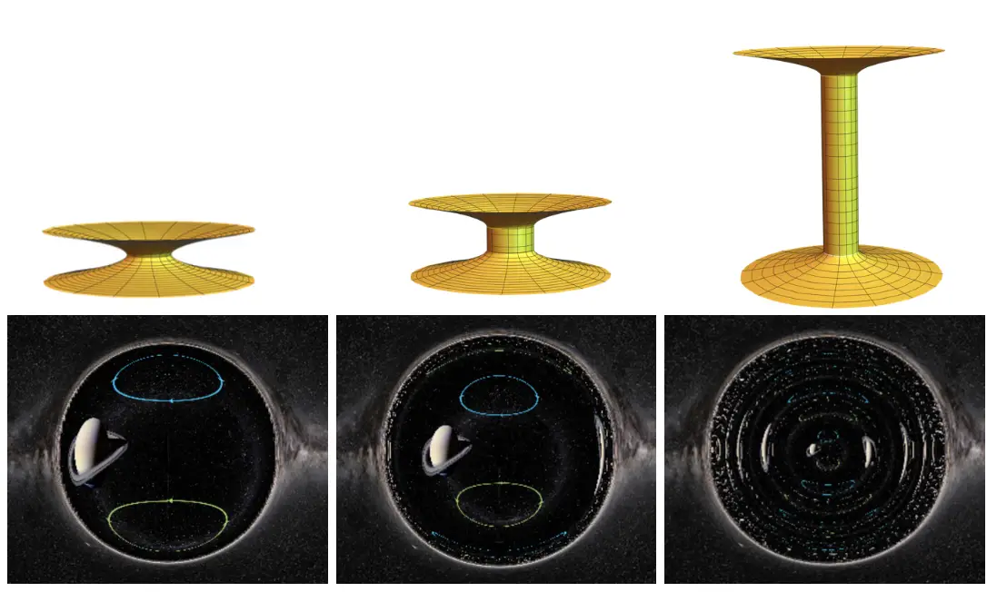
All of the images of these wormholes’ in Figure 6.2 appear with the Milky Way looking normal on the edges of the figures but the star field has been bent around the Einstein ring, the bright ring of light circling the wormhole. This distortion is similar to that seen in the images produced of Schwarzschild black hole. The stars are more densely packed in the lower celestial sphere image and less so on the upper in Figure 6.1, so it is easy to tell where the transition is between the wormholes mouth and its exterior, which causes brighter and darker areas on the image.

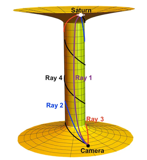
On the shortest wormhole of length $a=0.02$ the inner circular distorted primary image of Saturn is caused by the light rays taking the shortest route from the camera to the upper celestial sphere, which can be represented by ray 1 in Figure 6.3. The straight arrowed lines have been bent into oval shapes with the blue arrows circling in a clockwise direction and the green in an anti-clockwise direction. The faint star galaxy that first appeared along the line that a graph of cosine would make in the left Figure 6.1, but now makes a ring of stars on the inside of the wormhole’s mouth.

In the image of the wormhole of length $a=2$ the primary image of Saturn has moved closer to the centre of the throat and decreased in size. A secondary image of Saturn appears on the opposite side of the wormhole, that is more distorted this time and wraps more closely to the edge of the wormhole’s throat. This light travels along the second shortest path from the camera to Saturn, which wraps around the back of the wormholes throat as shown by ray 2 in Figure 6.3.

Increasing the length of this wormhole to $a=20$ causes several ray paths to end up at Saturn and so multiple distorted images appear. The images of Saturn again shrink and move closer to the centre with each new image of Saturn appearing on alternating sides of the wormholes mouth, becoming more distorted by becoming stretched and squashed. In Figure 6.3 we see four light rays all ending up at Saturn, and so this produces the four most central distorted images of Saturn in the wormhole’s mouth. Light paths spiralling the throat more times in various new directions cause the multiple versions on Saturn in the last image in Figure 6.2.

This proves that when the wormholes length is increased, this results in greater distortion on the wormhole’s mouth, in the images of the upper celestial sphere, and multiple distorted images are seen from the camera. The affect on altering the wormhole’s length is minimal for the image of the exterior of the wormhole’s mouth. We will now look at keeping the wormhole’s length constant and altering its lensing width.

6.2 Altering the Wormhole’s Lensing Width

Changing the wormholes lensing width increases the curvature of the embedded diagram between the wormhole’s throat and the celestial sphere. The embedded diagrams of wormholes with parameters $(\rho, \mathcal{W}, a)=(4,\mathcal{W} ,2)$, with $\mathcal{W}$ taking values of $(0.05,2)$, are shown in the top images of Figure 6.4. Their shape is displayed above their image appearance from the camera, which is set at a constant location of $(l_c,\theta_c, \phi_c)=(5, \pi/2, 0)$, which are represented by the bottom figures.

In both of the bottom images in Figure 6.4 the primary upper celestial sphere image in the centre of the wormhole’s throat is distorted in similar ways, with both of them appearing with similar size and shape because the length of the wormhole has been kept constant in both cases.

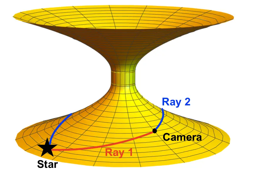
The wormhole with a small lensing width, $\mathcal{W}=0.05$, produces an image that only contains one visible clear primary image of both Saturn and the Milky Way, which has been caused by ray $1$ in Figure 6.5, that is bent around the wormhole. Nothing particularly interesting has happened here as not much distortion has occurred.

Whereas in the image of a wormhole with lensing width, $\mathcal{W}=2$, we see a secondary image of the Milky Way, caused by ray $2$ in Figure 6.5 that bends, from a star on the lower celestial sphere, around this curved exterior surface and still reaches the camera to produce a distorted image between the Einstein ring and the wormholes throat, which is similar to that of the Schwarzschild black holes image. This is repeated when looking into the wormhole’s throat, as both wormhole’s have the primary image of Saturn from the upper celestial sphere, but the wormhole with a greater lensing width also contains a secondary image of Saturn that has also been lensed towards the secondary image of the Milky Way in the wormhole’s exterior. This is as a result of it possessing a greater lensing width and hence more gravitational lensing occurs.

This Einstein ring appears the same as in the Schwarzschild black hole images. This is caused by the caustic on the celestial sphere that is opposite the camera, on the same side of the wormhole. If the camera was moved along the wormhole’s manifold, and the images were complied to produce a slow motion video, the stars near the Einstein ring would, again, move in opposite directions on either side of it, with the stars closer to the ring moving faster. This happens when the caustic point on the celestial sphere moves past other stars, due to the camera’s movement. When the caustic point is near a star, the rays that are produced by the caustic, which form the Einstein ring, are near the rays produced from the star, because their distance between them is small. This results in the star having a primary image just outside the Einstien ring and secondary image inside the other end of the ring. For this reason, primary images will always appear on the outside of the ring, and secondary, tertiary, and so on, on the inside of the ring.

Increasing the lensing width parameter increases the number of distorted images appearing of both of the celestial spheres, and hence is related to the amount of gravitational lensing that arises in the wormhole. We will now discuss what parameters the DN team chose to produce a clip of travelling through a wormhole.

6.3 Traveling through Interstellar’s wormhole

In the movie Interstellar, ^[14], Nolan got the DN team to analyse the wormhole’s images of various parameters, to chose the desired wormhole of length, $a=0.05 \rho$ and lensing width, $\mathcal{W}=0.05 \rho$. This small wormhole length was chosen so that the audience were not confused about the multiple distorted images in the interior. The lensing width was chosen to be much less than that of a Schwarzschild black hole to reduce the amount of gravitational lensing taking place, making it easier for the audience to depict the wormholes exterior from its interior.

The image of Saturn in Figure 6.1 was replaced by that of Interstellar’s distant galaxy, to make a more realistic video of travelling through the wormhole towards the distant galaxy. The length was chosen to be small because travelling through a long wormhole looked similar to travelling through a tunnel, which didn’t get the idea across to the audience that it was a shortcut through the higher dimensional bulk. Instead it appeared as though the camera was simply zooming in on the image of the upper celestial sphere, rather than travelling through the wormhole. In order to portray a sense of higher dimensions, the DE team developed a video visualising traveling past landscapes whilst approaching the distant galaxy at a fast speed.

We will now look into the effective potential of photons traveling through the Ellis wormhole geometry, to make a comparison with that of the Schwarzschild black hole geometry.

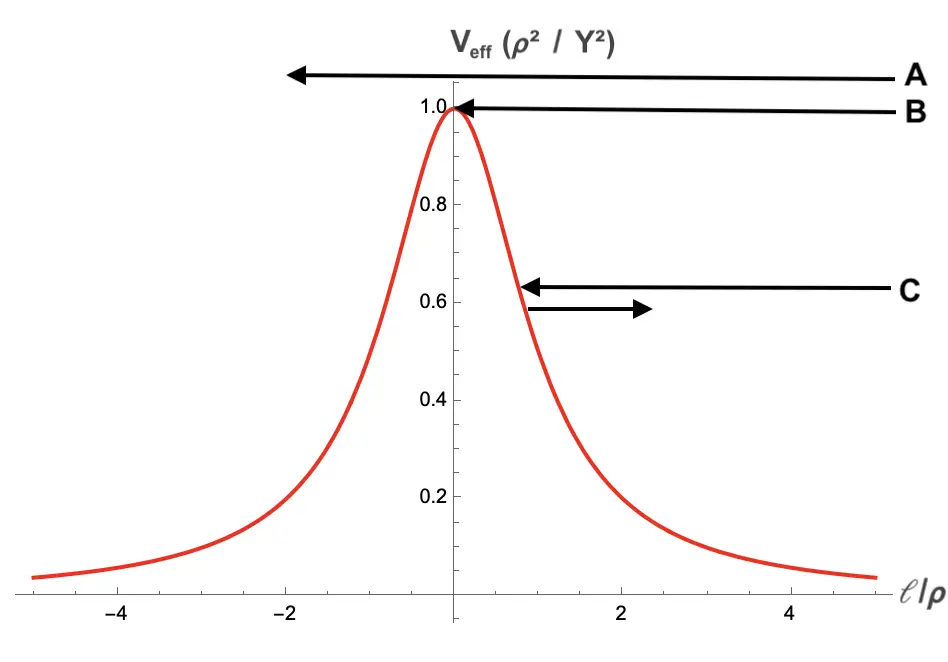
6.4 Effective Potential

The effective potential varies according to the nature of photon trajectories in the Ellis wormhole geometry. Work in this section has been based on that of Takayuki Ohgami and Nobuyuki Sakai, ^[13], Section IV. To derive an equation for the effective potential, we start by taking the null geodesic equation and setting the affine parameter as $\lambda$ and the null vector as $k^\mu \equiv dx^\mu/d\lambda$, with $k_\mu k^\mu=0$. This produces the following geodesics: $$\begin{aligned} \frac{d}{d\lambda}k^t &=0 , \\ \frac{d}{d\lambda}((l^2 + \rho^2)k^\phi) &= 0,\\ \frac{d}{d\lambda}k^l - l(k^\phi)^2&= 0,\\ -(k^t)^2 + (k^l)^2 +(l^2 + \rho^2)(k^\phi)^2&=0.\\ \label{4.20} \end{aligned}$$ Integrating the first two expressions above yields two conserved quantities, which are $$\begin{aligned} E&= k^t , \qquad Y= (l^2 + \rho^2)k^\phi.\\ \label{4.20b} \end{aligned}$$ The third expression in sequence of equations above can be derived using a combination of the other expressions, hence no conserved quantities are discovered from it. The last conserved quantity is found in the final expression , which becomes $$\begin{aligned} (k^l)^2 + V_{eff}(r) &= E^2,\\ V_{eff}(r) &= \frac{Y^2}{l^2 + \rho^2}.\\ \label{4.21} \end{aligned}$$

The effective potential, $V_{eff}(r)$, of photons in the Ellis wormhole geometry has been plotted against $l/\rho$, in Figure 6.7 and will be explained below. To find an expression for $dl/d\phi$, we combine equations above to give $$\begin{aligned} \frac{dl}{d\phi}&= \frac{k^l}{k^\phi} = \pm\frac{l^2 + \rho^2}{Y} \sqrt{E^2-V_{eff}}.\\ \label{4.21a} \end{aligned}$$ This equation encodes the photon’s spatial trajectories in the Ellis wormhole. As $r \to \infty$ the following limit is produced with $$\begin{aligned} \lim_{l \to \infty} \frac{1}{l^2} \frac{dl}{d\phi} &= \pm \frac{E}{Y}.\\ \label{4.22} \end{aligned}$$ This equation can then define the impact parameter, $b \equiv Y/E$. Plotting trajectories of photons of various natures, produces Figure 6.6, which contains the wormhole’s throat as the red circle, and photon trajectories of different natures, labelled $A, B$ and $C$. Trajectory $A$ passes through the wormhole, with its paths on the other side of the throat being represented by the dashed line. The $B$ trajectory orbits around multiple times while approaching the wormhole’s throat, which is shown in Figure 6.6. Photons on trajectory $C$ remain on one side of the wormhole and are bent from the curvature of the wormhole.

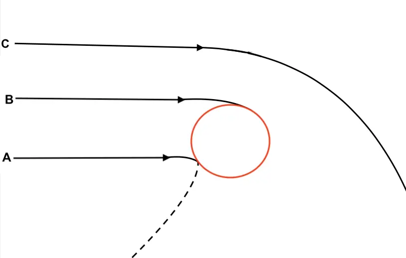
In the photons’ effective potential plot in Figure 6.7, the nature of these photons are demonstrated by Figure 6.6. The maximum potential of this diagram is in the centre of the wormhole’s throat, where $V_{eff} = Y^2/\rho^2$, which is represented by the trajectory $B$. This stationary point is an unstable orbit of photons as the slightest of changes of $l$ causes the potential of the photon to tend to zero. Trajectory $A$, has enough energy to pass over this potential barrier, hence it passes through the wormholes throat. Photons of this nature are responsible for producing the images of the upper celestial sphere, which is when the camera is on the other side of the wormholes throat, shown in the previous sections. Finally, trajectory $C$ does not possess enough energy to pass through the wormholes throat, hence it is only curved from it. These photons produced the images of the lower celestial while the camera is located on the same side of the wormhole. The further the photons get from the wormhole’s centre, the less potential they possess, as $l \to \pm \infty$ then $V_{eff} \to 0$.