Chapter 5: Ray Tracing in Wormhole Geometries

In this chapter we will discuss the existence of wormholes in our universe. The first wormhole discussed will be the Ellis wormhole, discovered by Homer Ellis, ^[6] in 1973. After the line metric and embedded diagram has been explained for this one parameter wormhole, we will move onto the three parameter wormhole that was produced by the DN team for the movie Interstellar, ^[14]. This new line metric will be examined so that equations of motion to ray trace in this wormhole geometry can be derived, to then produce a map from locations on a camera to a point on a celestial sphere. This will then be used in an algorithm to produce the wormhole images. Majority of the work in this chapter has been based on the work by the DN team’s paper, ^[7]. Where other sources have been used, they will be stated explicitly.

5.1 Introduction to Wormholes

A wormhole, also known as an Einstein–Rosen bridge, is a structure in spacetime that connects two parts of a universe together via a tunnel. This is seen in Figure 5.1 taken from Kip Thorne’s book, ^[8], Chapter 14, which shows two locations in the universe, $A$ and $B$, which are connected by the red dashed line in the real universe and by the blue dashed line through the wormhole. This implies that there is a shorter route from $A$ to $B$ then the actually distance between them in the universe.

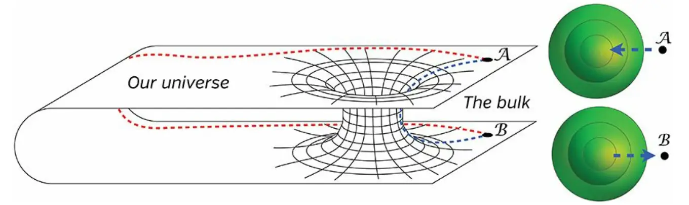
This curved structure connecting the two parts of the universe in Figure 5.1 is known as an embedded diagram of a wormhole. An embedded diagram expresses the shape of a four dimensional wormhole into a three dimensional curved manifold. This is because at each circle on this manifold’s surface there exists a sphere containing a circle as its cross section area, which represents the three dimensional space in the universe, hence one spatial dimension has been removed from the diagram. The diameter of these spheres’ on Figure 5.1 starting from location $A$ shrink in size when passing along the blue dashed line into the wormhole’s tunnel, until they reach the middle of the tunnel, which is where the sphere’s possess the smallest diameter. The diameter begins to grow in size when traveling through the bottom of the wormhole until they reach $B$.

Wormholes in our real universe have not been proven to exist. They are very likely to be forbidden by the laws of classical physics because of the presence of negative energy density inside them and the possibility of backward time travel. This negative mass has not been proven anywhere in the universe and hence if any photon or object was to enter the wormhole, it would collapse on them and the tunnel would pinch off. If this negative mass was possible, we would be dealing with a stable "traversable" wormhole that can stay open, and not pinch off. These are they type of wormholes we will be considering for the rest of the report. The first type of wormhole discussed will be the simplest one parameter wormhole, that does not have much freedom in controlling its shape.

5.2 The Ellis Wormhole

The Ellis wormhole is a simple wormhole that only possesses one parameter that affects its structure. Its metric was derived by Homer Ellis in 1973. The work below has been based on his work in ^[6]. This type of wormhole is known as a "drain hole" because it contains a vector field that is a velocity field for an ether draining through the hole. The line metric of this geometry is

$$\begin{aligned} ds^2 &= -dt^2 + dl^2 +r^2\left(d\theta^2 +\sin^2\theta d\phi^2\right). \\ \end{aligned} \label{4.1}$$ The function $r$ in the line metric is now defined as

$$\begin{aligned} r(l) &= \sqrt{\rho^2 +l^2},\\ \end{aligned} \label{4.2}$$ with $l , \phi \text{ and } \theta$ being the spherical coordinates as usual. The constant $\rho$ is related to the wormhole’s throat radius. This line metric in equation is of the same form as the Schwarzschild line metric found in the previous chapters, meaning that this type of wormhole, itself is also spherically symmetric making the metric similar to that of a Schwarzschild black hole because it contains the same $r^2(d\theta^2 +\sin^2\theta d\phi^2)$ term. The function $r$ here is the radius of the sphere at a point in space, but is determined by the above equation and depends on the coordinate $l$. The presence of the negative sign in $-dt^2$ proves that in this geometry with fixed coordinates, time increases in a time-like direction in an object’s proper time. The $dl^2$ term is another spatial coordinate that is an object’s proper radial distance that is independent of the other coordinates, due to the absence of cross coordinate terms like $d\phi dl$ or $d\theta dl$.

In Figure 5.2 an "embedding diagram" of the Ellis wormhole is shown. This shows the wormhole’s throat radius $\rho$, the coordinates $l\text{ and }\phi$ and the radius $r$. The one spatial dimension that has been removed from this diagram is the coordinate $\theta$, in the line metric equation, that makes each circle on the manifold surface into a sphere. When $l \to 0$ in equation r(l), where $r$ is expressed as a function of $l$, the value of $r \to \rho$ and when $l \to -\infty$ or $l \to \infty$ then $r \to |l|$. This explains the curvature in the embedded diagram when moving further away from the centre of the wormhole, as $r$ increases then so does $l$.

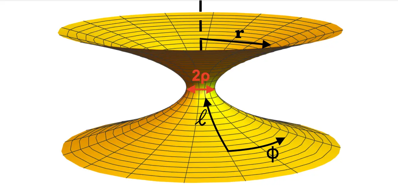
The shape of the Ellis wormhole cannot be altered as it only depends on one parameter, $\rho$. However, adding extra parameters to wormholes can then affect their shape, which is what is introduced in the next section.

5.3 The Three-Parameter Wormhole

Wormholes with more parameters are more desirable as there is more flexibility for altering the shape of them and hence the images produced. In the movie Interstellar, ^[14], directed by Christopher Nolan, the desired wormhole needed extra parameters to achieve the preferred images that appear when falling through a wormhole. So his team introduced the following parameters:

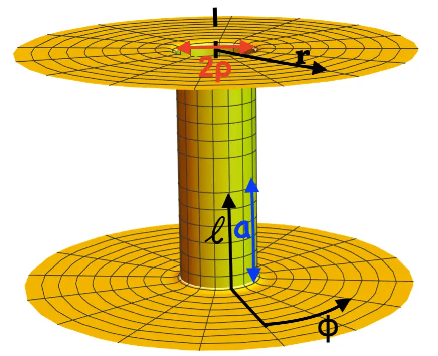
Firstly, a parameter measuring the length, $a$, of half of the wormhole’s interior, which is also the wormhole’s throat. This then turns out to produce a wormhole with very sharp transitions from the interior of the wormhole to the exterior. The line metric remains the same but the function of $r$ then becomes

$$\begin{aligned} r(l) &= \rho \text{ for the interior of the wormhole when } |l| \leq a ,\\ &= |l| -a +\rho \text{ for the exterior of the wormhole when } |l| > a .\\ \end{aligned} \label{4.3}$$ The embedded diagram for this two parameter wormhole appears as a cylinder, of length $2a$ and radius $\rho$, for the wormhole’s interior, and a flat three dimensional space on either side of the cylinder that excludes the cross sectional circle of the wormhole’s interior of radius $\rho$ as seen in Figure 5.3. These extremely sharp transitions would produce less accurate, bizarre images as no gravitational lensing would take place because the spacetime is flat on either side of the wormholes interior, which is why another parameter related to the curvature is added.

Secondly, a parameter known as the "lensing width" is added to the wormhole, which smooths the transitions from the interior, $|l| \leq a$ to the exterior, $|l| > a$, of the wormhole. This transition gives rise to gravitational lensing around the wormhole’s edges, causing multiple deformed images of stars to appear in the wormhole’s image. The transition of the wormhole was chosen to be similar to that of the horizon of the non-spinning Schwarzschild black hole covered in chapters two and three. The wormhole’s metric then becomes

$$\begin{aligned} ds^2 &= -\left(1-\frac{2M}{r}\right)dt^2 + \frac{1}{1-\frac{2M}{r}}dr^2 +r^2(d\theta^2 +\sin^2\theta d\phi^2). \\ \label{4.4} \end{aligned}$$ Here $dl$ has been replaced and now takes the form

$$\begin{aligned} dl^2 &= \frac{dr^2}{1-\frac{2M}{r}}.\\ \end{aligned}$$ To express $r$ as a function of $l$ the Interstellar team chose a simple analytical function similar to that of the Schwarzschild case with

$$\begin{aligned} r &= \rho +\frac{2}{\pi}\int_{0}^{\lvert l \rvert -a} \arctan{\left(\frac{2\xi}{\pi M}\right)} d\xi, \\ &= \rho +M[x\arctan{(x)} - \frac{1}{2}\ln(1+x^2) ], \text{ for } \lvert l \rvert > a,\\ \end{aligned} \label{4.4b}$$ and

$$\begin{aligned} r &= \rho \text{ for } |l| \leq a .\\ \end{aligned} \label{4.4c}$$ Where the function $x$ is defined as

$$\begin{aligned} x&\equiv \frac{\lvert l \rvert -a}{\pi M}.\\ \end{aligned} \label{4.4d}$$

To measure the amount of curvature we need to take into account the height of the embedded surface from the wormhole’s central mid plane, which slices through the interior cylinder. This change in height will be denoted as $dz$, and together the displacement $ds^2$ becomes $ds^2 = dz^2 + dr^2 + r^2d\phi^2$. Comparing this to the spatial metric of the two dimensional surface in the wormhole’s embedded diagram, that is $ds^2 = dl^2 + r^2(l)d\phi^2$, then proves that $dz^2 +dr^2 = dl^2$. Expressing this function of the height, $z$, in terms of the distance, $l$, through the wormhole gets $$\begin{aligned} z(l) &= \int_{0}^{l} \sqrt{1-\left(\frac{dr}{dl'}\right)^2} dl' .\\ \label{4.5} \end{aligned}$$

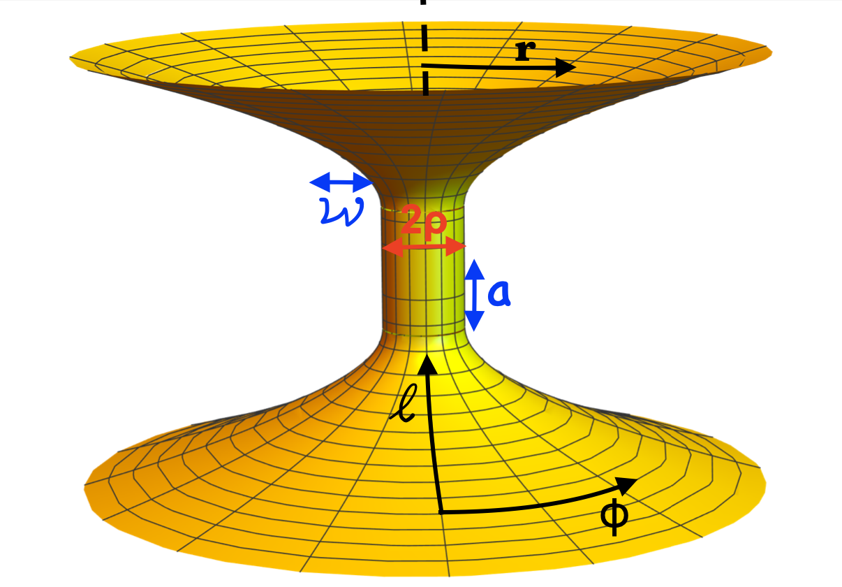
Substituting the functions of $r$ from the equations above into the above $z(l)$ equation, and coding this together with the line metric produces the embedded diagram of this three parameter wormhole shown in Figure 5.4. Here the lensing width parameter measuring the curvature is denoted by $\mathcal{W}$ and is related to a mass $\mathcal{M}$ by

$$\begin{aligned} \mathcal{W} &= 1.42953….\mathcal{M}.\\ \label{4.6} \end{aligned}$$

So $\mathcal{W}$ is actually a measure of the lateral distance in the embedding space, where the wormhole’s surface changes from being vertical at the interior to an angle of $45$ degrees on the exterior. The edges of the wormhole’s interior, at $l=\pm a$, is known as the wormhole’s mouth, which separates the interior from the exterior, which contains spheres of radius $\rho$. The shape of the wormhole’s embedded diagram in Figure 5.4 actually only depends on the two ratios, the first being the mass-to-radius, $\mathcal{M}/\rho$, and the second being the length-to-diameter , $2a/2\rho= a/\rho$.

Now that we have an understanding of the different types of wormhole’s line metrics and embedded diagrams, we can start looking at how the code produces these embedded diagrams.

5.4 Producing the Embedded Diagrams

This data has been written based on the work of Jason B,^[11].

To program the wormhole’s embedded diagram, the functions, $x,r$ and $z$, of $l$ will be used. The function of $x$ and $r$ come from expressions in equations above to give

$$\begin{aligned} x&\equiv \frac{\lvert l \rvert -a}{\pi M},\\ r &= \rho +M[- \frac{1}{2}\ln(1+x^2) + x\arctan{(x)} ], \text{ for } \lvert l \rvert > a,\\ r &= \rho \text{ for } |l| \leq a .\\ \end{aligned} \label{4.13a}$$ The expression for $dr/dl'$ is given by differentiating equations for $r$ above with respect to $l$ to get $$\begin{aligned} \frac{dr}{dl'} &= 0 , \text{ for } |l| \leq a ,\\ \frac{dr}{dl'} &= \frac{2}{\pi} \arctan{\left(\frac{2(\lvert l \rvert -a)}{\pi M}\right)}, \text{ for } \lvert l \rvert > a.\\ \label{4.13c} \end{aligned}$$ Substituting this expression for $dr/dl'$ into the function for $z$ taken from equation of z(l) produces $$\begin{aligned} z(l) &= 0 , \text{ for } |l| \leq a,\\ z(l) &= \int_{0}^{l} \sqrt{1-\left(\frac{2}{\pi} \arctan{\left(\frac{2(\lvert dl' \rvert -a)}{\pi M}\right)}\right)^2} dl' , \text{ for } \lvert l \rvert > a.\\ \end{aligned} \label{4.13a}$$ The code uses these functions to produce the embedded diagram using polar coordinates that are translated into cartesian coordinates with $\{x,y,z\} = \{r\cos{\theta}, r\sin{\theta}, \pm z\}$, which is representing both sides of the wormhole because $z$ takes both positive and negative values for $\theta \in (0,2\pi)$. It then produces the plot after entering the wormhole’s parameters $(\rho, \mathcal{W}, a)$.

Now that the code has been explained to display the shape of wormholes by plotting their embedded diagrams, we will start explaining how these images of wormholes are produced.

5.5 Images of Wormholes

To produce images of wormholes’ a camera is placed at a desired position, either in the interior of the wormhole or exterior, and then absorbs light from different directions to produce the image. To simplify our model, it is now assumed that the only source of light is coming from the upper celestial sphere and the lower celestial sphere. These celestial spheres are also assumed to be lying at $l\to +\infty$ and $l\to- \infty$ respectively on the wormhole. A camera that is located at the black dot in Figure 5.5 can capture light from both null geodesic light rays labelled ray $1$ and ray $2$. The light from ray $1$ is coming from the upper celestial sphere and for ray $2$ from the lower, hence the camera will produce an image of the wormhole that contains distorted images of both celestial spheres.

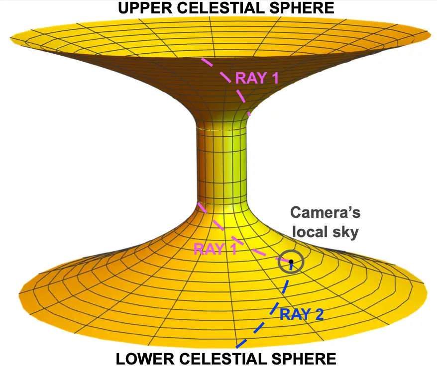
To depict exactly where this light is coming from on each of these celestial spheres the coordinates of this light will be labelled, when $l \to \pm \infty$, as $\{ \theta', \phi'\}$ on one of the spheres. Light rays will be traced backwards for each direction, $\{ \theta_{cs}, \phi_{cs}\}$, on the camera’s local sky until $l \to \pm \infty$, where they will end at the location $\{ \theta', \phi',s \}$ on one of the celestial spheres. To know which celestial sphere the light has travelled from, the sign $s$ is analysed. If it is positive, the light has come from the upper celestial sphere and if it is negative, it has come from the lower. As in the previous chapter with ray tracing Schwarzschild black holes, the image of the point emitting light on the celestial sphere will appear from the direction the light ray enters the camera’s local sky, but will appear distorted. Producing a map from $\{ \theta_{cs}, \phi_{cs}\} \to \{ \theta', \phi',s \}$ is the key to producing images of the wormholes.

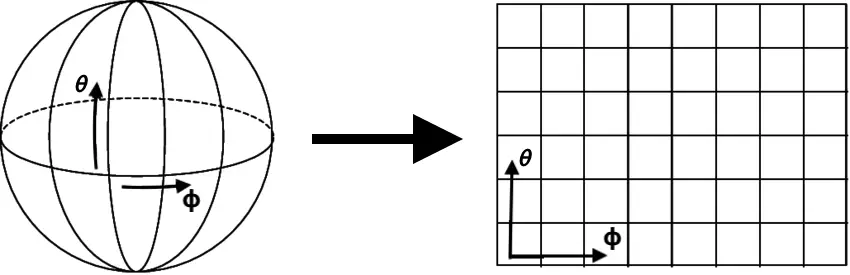
To produce pictures of wormholes we need to understand how images of spheres appear in flat two dimensional images. The images of the celestial spheres’ that are attached to the code will be flat photos, which is made possible by a longitude-latitude mapping system. This is the same system that is used when viewing the earth on a map that is a two dimensional photo. It converts the angle, $\{ \theta, \phi\}$, on a sphere to become the pixel, $\{ \theta, \phi\}$, on the flat image as shown in Figure 5.6. Here the angles take the values of $\phi \in (0,2\pi)$ and $\theta \in (0,\pi)$.

Now that we have an understanding of how light travels from the celestial spheres to a camera’s local sky, we can move onto deriving the geodesic equations that photons moves along in the wormhole’s geometry.

5.6 The Equations of Motion

We need to derive a system of differential equations that trace the paths along which light moves from the camera to the celestial spheres. This can then be used to produce images of the wormholes.

The light travels along null geodesics in the wormhole’s spacetime, hence we need to find solutions to the geodesic equations,

$$\begin{aligned} \frac{d^2 x^\alpha}{d\zeta^2} +\Gamma^\alpha_{\mu\nu}\frac{d x^\mu}{d\zeta} \frac{d x^\nu}{d\zeta}&=0,\\ \end{aligned} \label{4.71}$$ that were derived in a previous equation. Here the affine parameter $\zeta$ will be used, which varies along these geodesics. We write these geodesics in the Hamiltonian language form, rather than the Euler-Lagrange form that we used to find the geodesics in Chapter 2. This is a better method as the structure of manifolds for wormholes are explained more precisely in this way, so we use the Hamiltonian formula $$\begin{aligned} H(x^\alpha, p_\beta) &= \frac{1}{2} g^{\mu\nu} ( x^\alpha ) p_\mu p_\nu \\ \end{aligned}$$ where our photons coordinates, $x^\alpha$, possess a generalised momentum, $p_\alpha$. The inverse of our metric is still denoted by $g^{\mu\nu}$ that keeps $H$ invariant under the change of coordinate systems. The Hamilton equations with respect to $\zeta$ are then

$$\begin{aligned} \frac{dx^\alpha}{d\zeta} &= \frac{\partial H}{\partial p_\alpha} = g^{\alpha\nu} p_\nu ,\\ \frac{dp^\alpha}{d\zeta} &= -\frac{\partial H}{\partial x_\alpha} = -\frac{1}{2} \frac{\delta g^{\mu\nu}}{\delta x^\alpha} p_\mu p_\nu .\\ \label{4.7} \end{aligned}$$ Using the above equations, the Hamiltonian can be proven to be constant along geodesics. Taking the derivative of $H$ with respect to $\zeta$ yeilds $$\begin{aligned} \frac{d H}{d \zeta} &= \frac{\partial H}{\partial x^\alpha} \frac{dx^\alpha}{d\zeta} + \frac{\partial H}{\partial p^\alpha} \frac{dp^\alpha}{d\zeta}, \\ &=- \frac{dp^\alpha}{d\zeta} \frac{dx^\alpha}{d\zeta} + \frac{dx^\alpha}{d\zeta} \frac{dp^\alpha}{d\zeta} =0.\\ \end{aligned}$$ This derivative of the Hamiltonian being equal to zero proves that is it constant and hence solves the geodesic equations. Dividing the momentum coordinates of the Hamiltonian by their corresponding coefficient functions in the line metric equation derives the super Hamiltonian of the wormhole’s metric, which becomes $$\begin{aligned} H &= \frac{1}{2} [-p_t^2 +p_l^2+\frac{p_\theta^2}{r(l)^2} +\frac{p_\phi^2}{r(l)^2 \sin^2\theta}] .\\ \label{4.8} \end{aligned}$$ Both $\phi$ and $t$ are missing from this equation, so this implies that $p_t$ and $p_\phi$ are both conserved quantities along a ray. We then denoted $p_\phi$ by $$\begin{aligned} b &= p_\phi, \\ \end{aligned}$$ where $b$ is a constant related to the photons impact parameter relative to the polar axis of the wormhole. The other conserved quantity $p_t$ satisfies $p^t= dt/d\zeta = -p_t$, hence $p_t$ has to be set to $p_t=-1$ so that it is conserved. This causes $\zeta=t$, which will be implemented later in equations, because $$\begin{aligned} \frac{dt}{d\zeta} &= -p_t =1.\\ \end{aligned} \label{4.8a}$$ Another conserved quantity is the photon’s angular momentum, which is related to the photon’s impact parameter, $B$, to the the wormhole’s centre, because of the spherical geometry. This constant $B$ then equates to $$\begin{aligned} B^2 &= p_\theta^2 + \frac{p_\phi^2}{\sin^2\theta}.\\ \end{aligned}$$ The following ray equations are derived by solving the Hamilton equations using the wormholes Hamiltonian in equation and the relation between $\zeta$ and $t$ in above equation which gives

$$\begin{aligned} \frac{dl}{dt} &= p_l,\\ \frac{d\theta}{dt} &= \frac{p_\theta}{r^2},\\ \frac{d\phi}{dt} &= \frac{b}{r^2\sin^2\theta},\\ \frac{dp_l}{dt} &= \frac{B^2\frac{dr}{dl}}{r^3},\\ \frac{dp_\theta}{dt} &= \frac{b^2\cos\theta}{r^2\sin^3\theta}.\\ \label{4.8b} \end{aligned}$$ These equations encode the photon’s trajectories along the geodesics as a function of time, with coordinates $\{l,\theta, \phi, p_l, p_\theta \}$. Now that these equations have been found we can produce a code that ray traces these photons to produce a map from $\{ \theta_{cs}, \phi_{cs}\} \to \{ \theta', \phi',s \}$.

5.7 Mapping a Point on the Camera to the Celestial Spheres

To produce this map from a point on the camera’s local sky to one of the celestial spheres, the following steps are needed.

• Firstly, the location of the camera is chosen depending on the desired output, which has coordinates denoted by $(l_c,\theta_c, \phi_c)$. This is normally set at $\theta_c =\pi/2$ to reduce the chance of getting a coordinate singularity at $0$ or $\pi$.

• Secondly, we set the origin at our camera’s location and for every point on the camera’s local sky $(\theta_{cs}, \phi_{cs})$, the following normal vectors are calculated to transform them into Cartesian form by setting

  $$\begin{aligned} N_x &= \sin\theta_{cs} \cos\phi_{cs} , \qquad N_y &= \sin\theta_{cs} \sin\phi_{cs} , \qquad N_z &= \cos\theta_{cs}. \\ \end{aligned}$$ The unit vectors $(\bm{e_x} ,\bm{e_y}, \bm{e_z} )= (\bm{e_{\hat{l}}} ,\bm{e_{\hat{\phi}}}, -\bm{e_{\hat{\theta}}} )$ are pointing in the $l,\phi,$ and $-\theta$ directions respectively. This minus sign on the $\theta$ component is chosen so that when $l$ is positive, the wormhole’s polar axis is parallel to $\bm{e_z}$, from the upper celestial sphere. The photons are incoming into the camera from a direction of $-\bm{N}$, because of the backwards ray tracing, so then the vector representing the true direction of photons, $\bm{n}$, becomes the following: $$\begin{aligned} n_{\hat l} &= -N_x, \qquad n_{\hat \theta} &= -N_y, \qquad n_{\hat \phi} &= +N_z. \\ \end{aligned} \label{4.10}$$

• Using the values in equation above to calculate the photons canonical momenta that are defined by $$\begin{aligned} p_{l} &= n_{\hat l}, \qquad p_{\theta} &= r n_{\hat \theta}, \qquad p_{\phi} &= r\sin\theta n_{\hat \theta}. \\ \end{aligned} \label{4.11}$$ After these values of the momentum have been calculated, then compute the constants photon’s constants of motion, $b$ and $B^2$, that were derived in the last section as

  $$\begin{aligned} b &= p_\phi = r\sin\theta n_{\hat\phi},\\ B^2 &= p_\theta^2 + \frac{p_\phi^2}{\sin^2\theta} = r^2(n_{\hat\theta} +n_{\hat\phi}).\\ \end{aligned} \label{4.12}$$

• Using these expressions in equations above, integrate the equations of motion in , to produce an array of locations of photons’. Using these results, create arrays of $\{ \theta_{cs}, \phi_{cs}\}$ and $\{ \theta', \phi',s \}$ values, so that an interpolating function in Mathematica that compares these corresponding values and creates a map between then. So that for any value of $\{ \theta_{cs}, \phi_{cs}\}$ entered, it calculates the corresponding $\{ \theta', \phi',s \}$ value.

Using these steps, any point on the camera’s local sky can have a photon path traced backwards to where it came from on one of the celestial spheres. Now that we have this mapping we can start looking into the algorithm used to produce images of these wormholes.

5.8 The Backwards Ray Tracing Algorithm

This data has been written based on the work of Jason B,^[11].

The code can then produce images of the three-parameter wormhole. It consists of the following backwards ray tracing algorithm to produce images:

• Set the three parameters for the desired wormhole $\{\rho, a, \mathcal{W}\}$ and the position of the camera’s local sky with coordinates $\{l_c,\theta_c, \phi_c\}$, and the images of the celestial spheres are attached.

• Produce the mapping of $\{ \theta_{cs}, \phi_{cs}\} \to \{ \theta', \phi',s \}$ using this camera’s location and the parameters of the wormhole. This mapping has been derived in the previous section. In the code the functions of $l$, the canonical momenta and the constants of motion have been defined. The differential equations of motion, have been solved, that takes the initial values and solves backward in time to ray trace the photons. The actual map is then defined in a function, that ray traces the photons and then stores the values of $\{ \theta', \phi',s \}$ for the corresponding $\{ \theta_{cs}, \phi_{cs}\}$.

• The final function labeled "wormhole" uses an interpolating function to produce the image of the wormhole by using the mapping from $\{ \theta_{cs}, \phi_{cs}\} \to \{ \theta', \phi',s \}$ for each pixel, $\{\theta_{cs}, \phi_{cs}\}$, on the camera’s local sky. The colour of the pixel should be taken from the upper celestial sphere if $s$ is positive and from the lower if $s$ is negative.

Now that we have the equations of motion of photons in a wormhole’s spacetime and the code that uses the algorithm to produces images of them, we can start analysing why they appear as they do.