Chapter 4: Schwarzschild Black Hole’s Appearances and Properties

Using the equations of motion and coding algorithm derived in the last chapter we will now produce the images of black holes and explain why they appear as they do. To do this we start by explaining how the concept of gravitational lensing distorts the images in specific ways. We will relate this property to the Schwarzschild black hole images and evaluate why they appear as they do, explaining the appearance of the Einstein ring and event horizon. We will finally look into the black hole’s singularities and the effective potential energy that the photons possess. Throughout this chapter we will mainly be using work based on the gravitational lensing paper written by the DN team in, ^[4], Section 3 and Shultz,^[1], Chapter 11.1. The other sources will be stated explicitly in the relevant section.

4.1 Gravitational Lensing

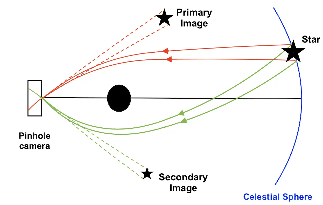
Gravitational lensing is when photons from an object travel in different directions around a black hole and intersect again in the future due to their curvature in spacetime. When a single object emits multiple light rays that reach the same point on a camera’s aperture, multiple images of the object appear in the camera’s distorted image. This is seen in Figure 4.1 where light from a star on the celestial sphere, curves on either side of the black hole and both light trajectories end in the pinhole camera. Two images of the same star are seen from the camera’s perspective and they appear in different directions and are distorted in size and shape. The light that takes the path of shortest distance produces the "primary image" of the star, and the next shortest path of light traveling in the opposite direction around the black hole produces the "secondary image", which is smaller in size. Multiple distorted images of objects can appear because of this. With this knowledge we can comprehend the way light moves around these black holes.

4.2 Image Analysis and the Einstein Ring

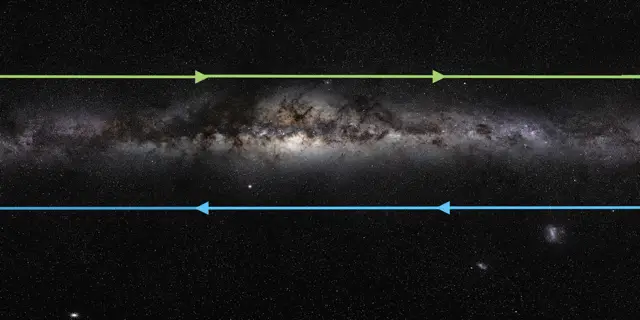
The image in Figure 4.2 is a picture of the Milky Way that has been used as the celestial sphere behind the black hole in our model. This image has been taken by Serge Brunier, ^[9], which we have added two coloured lines with arrows on them to make it easier to depict where some parts of the star field have been deflected to and how their appearance is distorted in the final image. Using the coding algorithm in the last chapter, our code produces the distorted image in Figure 4.3 of a Schwarzschild black hole with a mass of $M=2.5$, and the camera’s location set to $r_{\tau=0} = 22$, $\phi_{\tau=0}=\frac{\pi}{2}$.

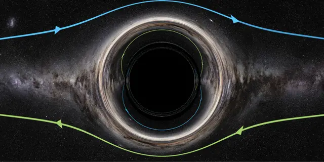
The circular black disc in the centre of Figure 4.3 is known as the black hole’s event horizon, which is the boundary of the black hole itself. It is a "boundary in spacetime separating events that can communicate with distant observers and events that cannot" stated from Shultz’s, ^[1], Chapter 11.3. After any light-like or time-like geodesics fall below the event horizon they will never be able to escape out of it again, as they have been trapped by the black hole. The event horizon has a Schwarzschild radius of $R_s = \frac{2GM}{c^2} = 2M$. For this reason the black hole appears as a black disk because all the light coming from that direction has been absorbed by it and cannot escape. This explains why the plot in Figure 3.4 has no corresponding $\alpha'$ values for small $\alpha$ values as the photons had been absorbed by the black hole.

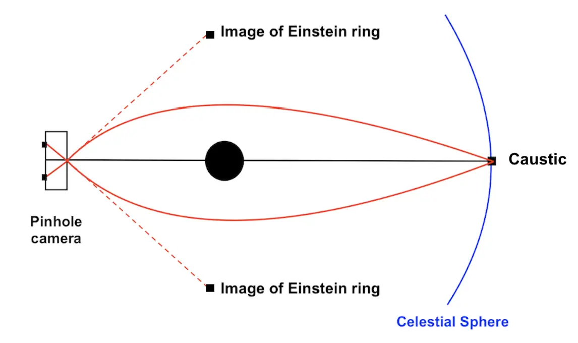
The outer bright ring shown in Figure 4.3 is known as the Einstein ring, which is an image of whatever star constellation is directly behind the black hole from the pinhole camera. This point on the celestial sphere is known as the caustic point. This bright ring appears as our star constellation has a high density of bright stars behind the black hole. The light from these stars obviously cannot reach the camera from travelling in straight lines, instead the light paths curve around the black hole along symmetric paths in all directions, hence they make a perfect ring of light in our image. This is caused by gravitational lensing shown in Figure 4.4 when there is perfect alignment of the camera, black hole and the caustic. When we generalised our two dimensional model to three by introducing the angle $\beta$, the rotation of this equational plane in Figure 4.4 clearly ends up producing the perfect ring of light from the camera’s perspective caused by the caustic point.

Something particularly interesting happens at this ring, when the images are zoomed in. Multiple images are taken while the camera is slowly moved. Compiling these produce a short slow motion clip showing the stars on one side of the ring are travelling rightward, and stars on the other side travel leftward. The closer the stars are too the ring the faster they move around it, this results in the stars near the ring to appear very stretched, which is due to their high speeds. This is shown in the video by Thomas Müller, ^[12], where a black hole is moving in front of the Milky Way image by Brunier, ^[9].

In Figure 4.3, outside the Einstein ring we see the "primary image" of the Milky Way galaxy that has been, as expected, inverted horizontally and vertically, proven by the arrows changing direction and orientation. This image has also been stretched around the Einstein ring and slightly deflected away from it, this deflection happens as a result of the gravitational lensing from the red light rays in Figure 4.1, which travel along the shortest path possible from the celestial sphere to the camera in this geometry.

Just outside of the event horizon and inside the Einstein ring is a small distorted "secondary image" of the Milky Way appears upside down and inverted again. The arrows now loop from the event horizon towards the Einstein ring and loop, in the opposite direction to the primary images, to the other side of the Einstein ring and then back towards the event horizon. The light paths responsible for this distortions are shown in Figure 4.1 by the green paths, where the light has travelled in the opposite direction around the black hole before reaching the camera.

A much fainter version of the Milky Way, known as the "tertiary image", then wraps around closer to the event horizon because it is much smaller with a lot dimmer light. Depending on the parameters chosen in the program different distortions of these images are curved in this area. However the two rays in the gravitational lensing Figure 4.1 does not explain why there are more than two distorted images appearing that are wrapping closer to the event horizon. This tertiary image appears because photons from the same object causing the primary and secondary images in Figure 4.1 travel along new paths over the top of the black hole that are close enough to it that they are curved around to circle the entire black hole, turning a full $360$ degree loop, and still end up entering the pinhole camera. The same is repeated on the lower side of the black hole, producing a "quaternary image". Moving in closer towards the event horizon, multiple distorted versions of the Milky Way appear as the photons paths that are very close to the black hole can start doing multiple loops around it. In Figure 4.3 we see they appear on alternating sides on the event horizon, as the photons paths alternate which direction they travel around the black hole, and shrink in size, as the paths become nearer to each other after looping around it. This can be seen more clearly with altering the parameters.
But how many times can a photon orbit a black hole and how close can they can get to a it before they pass a point of no return, leading them to being trapped by the black hole?

4.3 The Impact Parameter and the Photon Sphere

To find out how close a photon can get to a black hole, we need to consider the energy that a photon possesses. Work from this section to derive the impact parameter has been taken from Hobson’s book, ^[2], Chapter 9.13.

Using the photon’s potential equation with the expression of $E^2$ being replaced by $1/b^2$ where $b$ is an impact parameter produces: $$\begin{aligned} \dot{r}^2 &= E^2(r) - V_{eff}(r), \\ \dot r^2 + V_{eff}(r) &= \frac{1}{b^2},\\ V_{eff}(r) &= \left(1-\frac{2M}{r}\right) \frac{1}{r^2}.\\ \end{aligned} \label{4.0aa}$$ The angular momentum, $L$, of a photon has been ignored in the potential equation in the bottom of the equations above. Using the value of $\dot{\phi}$ from the previous chapters equation and dividing by the above expression of $\dot{r}$ from the top equation above gives $$\begin{aligned} \frac{d\phi}{dr} &= \frac{\dot{\phi}}{\dot{r}} = \frac{1}{r^2}\left( \frac{1}{b^2}-\frac{1}{r^2} \left(1-\frac{2M}{r} \right) \right)^{-1/2}.\\ \end{aligned} \label{4.0a}$$ For photons orbiting, as $r \to \infty$, our equation becomes $$\begin{aligned} r^2\frac{d\phi}{dr} &= \pm b.\\ \end{aligned} \label{4.0b}$$ Assuming that when $r\to \infty$ this causes $\phi \to 0$, then we get a solution for $b$ as $$\begin{aligned} b &= \mp r\sin{\phi}.\\ \end{aligned} \label{4.0c}$$

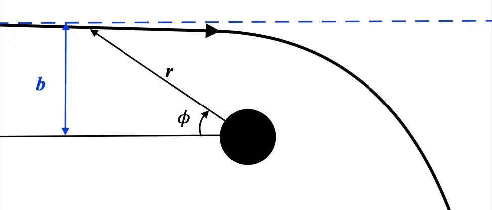
The impact parameter, $b$, now denotes the vertical distance, between the equatorial plane that passes through the centre of black hole, and a photon that is horizontally approaching the black hole from infinity, as shown in Figure 4.5. To understand how close photons can get to a black hole without being absorbed by them, light rays are traced by shooting photons horizontally towards the black hole at different values of $b$. Observing this from a perpendicular point of view, the Figure 4.6 is seen, so that we can evaluate how close the photon’s path can get and at what values the nature of these orbits change.

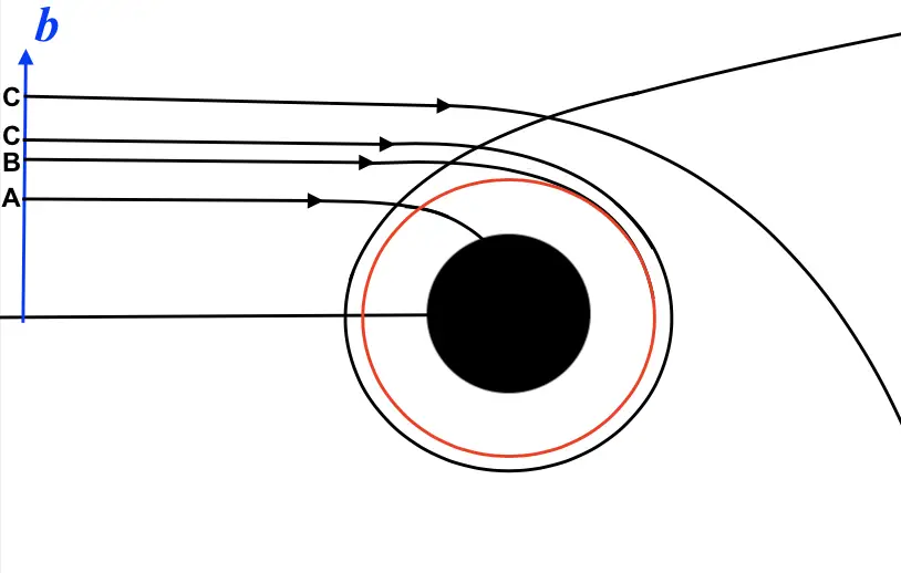
Starting the photons being shot at a height of $b=0$, to the height of the event horizon, $b=2M$, shown as the black disc’s height, the photons will clearly be absorbed, as in Figure 4.6. The photons traveling at $b < 3\sqrt{3}M$ curve inwards over a ring called the photon sphere, represented by the red ring, and then continue to curve over the event horizon and disappear into the black hole. Both of these cases can be described by ray $A$ in Figure 4.6. This photon sphere has radius $b =1.5R_s= 3M$. It acts as a point that once a free falling orbit passes over it, from the outside to the inside, the photon will then spiral into the event horizon.

In Figure 4.6 where light ray $B$ is shot parallel at $b = 3\sqrt{3}M$, the photons curve just enough to orbit multiple times to get infinitesimally close to the photon sphere, represented by the red ring, but never cross it. For this reason images of black holes appear bigger than the actual Schwarzschild radius. Photons travelling at a distance of $b>3\sqrt{3}M$, shown as both of the light rays labelled $C$, have paths that are not close enough to the black hole to be absorbed by it, hence they escape away from the black hole and travel back to infinity.

Values of $b$ that are greater than but very close to $3\sqrt{3}M$, cause the photons to approach this photon sphere just enough to just trace it while orbiting it multiple times and then still manage to escape. Light from a celestial sphere that reaches the camera after orbiting the black hole will cause another distorted image appearing just outside the event horizon. This explains the appearance of the tertiary and quaternary distorted images appearing so close to the black disc in Figure 4.3. So light from the Milky Way is now traveling in either direction around the black hole, orbiting near the photon sphere, and ending at the camera, hence causing multiple faint thin distorted versions of the Milky Way to appear.

The nature of these orbits around the black holes can be related to their potential energy of their photons.

4.4 Effective Potential

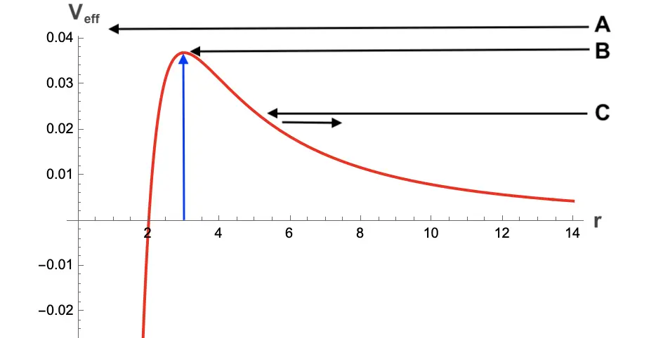
In this section work is based on the work of Harsha Miriam Reji and Mandar Patil ^[5] and from Hobson ^[2], Section $9.13$. Taking the equation of the effective potential energy, $V_{eff}$, in the expression for effective potential above, without the angular momentum gives $$\begin{aligned} V_{eff}(r) &= \left(1-\frac{2M}{r}\right) \frac{1}{r^2}.\\ \end{aligned} \label{4.1}$$ Plotting the potential against the radius, $r$, produces Figure 4.7. Finding the derivative of the potential with respect to the radius, which is also the gradient of the plot, gives $$\begin{aligned} \frac{dV_{eff}(r)}{dr} &= \frac{2(3M-r)}{r^4},\\\ \frac{dV_{eff}(r)}{dr} &= 0 \text{ at } r = 3M = 1.5 R_s\text{ with the maximum value of }\\ V_{eff}(3M)= \frac{1}{27M^2}.\\ \end{aligned} \label{4.2}$$

On the graph in Figure 4.7 we see the curve starts having non-negative potential at the event horizon $r=R_s=2M$, where the effective potential of a photon is zero. The effective potential then goes up to a maximum at $r=3M$ where the photon sphere is, with $E_p=1/27M^2$, shown by the blue arrow. This is the only turning point because it is the only solution when the derivative of the potential with respect to the radius is equal to zero. It is an unstable stationary point because all orbits near the photon sphere are unstable, as a tiny change in the orbit will cause the photon’s potential to drop drastically. As $r$ increases after this, $V_{eff} \to 0$ as $r\to \infty$, because it becomes a flat spacetime far away from the black hole. And the following limits therefore exist: $$\begin{aligned} \lim_{r \to 0} (V_{eff}) &= -\infty ,\\ \lim_{r \to \infty} (V_{eff}) &= 0.\\ \end{aligned} \label{4.3}$$

Any photon with $V_{eff} > \frac{1}{b^2}$ has enough potential to cross this potential barrier, the photon sphere, and then enter the event horizon and is absorbed by the black hole, which are labelled $A$ in both Figure 4.7 and Figure 4.6. If the photon’s potential is $V_{eff} = E^2 = \frac{1}{b^2}$ it will just trace the photon sphere and can continue to orbit infinitely many times, because the angular velocity is not equal to zero, represented by ray $B$. At this orbit we have $1/b^2 = 1/27M^2$, hence the value of the impact parameter is $b=3\sqrt{3}M$. This is the reason the value of $b$ used in the last section was the turning point for the change in nature of the photon’s orbits, from being deflected away from the black hole, to being absorbed by it. At $V_{eff} < \frac{1}{b^2}$ the photon is curved by the black hole but will never have enough potential to pass over the photon sphere, hence it will be deflected away and escape back to infinity, represented by ray $C$ in both figures.

But we wonder where this energy is transferred to when light and objects pass into the black hole?

4.5 Singularities

The line metric equation fails at both $r=0$ and at $r=2M$, which causes two singularities. Work from this section has been taken from Shultz’s, ^[1], Chapter 11.2.

There always exists a spacetime singularity in the centre of the black hole where all objects are absorbed to, this has the entire mass of the black hole, $M$, contained in an infinitely small space with radius, $r=0$, causing the density of this point to be infinite. This is where all objects and photons end up at after crossing over the event horizon, which can not be seen by external observers that are outside the black hole because not even photons can escape out of the event horizon again. At this point the gravitational field is so strong that the spacetime itself is broken down, which causes the curvature of the manifold to be infinite.

At $r=2M$ there exists a coordinate singularity, which is caused by the coordinate system failing because it does not define this part of the geometry properly, rather than the black hole having a singularity at this location. Change of coordinate systems can eliminate this failure. The equations cannot be defined at these points, hence they are ignored in the line metric, causing the line metric in this geometry to only be defined outside of the event horizon.

Now that we have discussed various properties of these black holes, we can start considering the next type of spacetime geometry, the wormhole geometry.