Chapter 3: Ray Tracing in the Schwarzschild Geometry
The Schwarzschild black hole is a spherically symmetric,
non-rotating, charge-less black hole that was discovered by Karl
Schwarzschild in 1915. For these reasons it is the simplest type of
black hole. In this chapter we will derive the line metric of the empty
space around this black hole’s body, followed by the equations of motion
for photon’s trajectories around it. We will then write up a piece of
code made in python that contains an algorithm that produces distorted
images of these black holes.
3.1 The Schwarzschild Metric
The trajectory of photons around Schwarzschild black holes are governed by its line metric. This line metric is derived below using solutions of Einstein’s field equations. The work below has been based on Hobson’s book [2], chapter , Sections and .
Because we are dealing with a spherically symmetric geometry, we use the spherical coordinate line metric form of Minkowski space, derived in the previous chapter. It now also consists of multiplying each of the terms by arbitrary coefficient functions of and to make this line metric unique to this Schwarzschild geometry, which are our metric functions, . So the line metric becomes The spherically symmetric geometry means that the only spatial coordinate that is affected by the gravitational field force is the radial coordinate, , so by taking a new coordinate system of , it is found that the function . The line metric needs to be invariant under changing the time component from positive to negative, , because the geometry is at rest. This causes the coefficient multiplied to to equate to zero, hence we have . This also requires our functions to be independent of the time-like coordinate, , turning the line metric into
The line metric now satisfies the form of a spacetime metric that is static spatially isotropic because all of its terms are invariant under rotation of its space-like coordinates and all of its terms, except for the time-like coordinate, are independent of time.
To find expressions of the functions a unique solution of the Einstein’s equations needs to be determined. Starting with the Ricci tensor, we find that it vanishes in empty space because of the absence of matter, which only contains a gravitational field, so we have the Ricci tensor as Equating the Riemann curvature equation with the Ricci tensor equation we obtain with our Christoffel symbol, , as before having a relation with the metric, , equation as The calculus tensor method of solving the Einstein equations is done by directly calculating from our equation, using the values of , where we have our expressions of and taken directly from the line metric equation to give Using these values of and substituting them into equation gives the first non-zero Christoffel symbol, , as Repeating this for all of the Christoffel symbols, we find that there are only 9 non-zero elements of the 40 independent connection coefficients, with them being The Ricci tensors are then calculated tediously by substituting these Christoffel symbols into equation. Substituting in the relevant expressions gives the first Ricci tensor as All of the non-diagonal components of the Ricci tensors equations equate to zero, when , giving the diagonal terms as Equating the Ricci tensor equations to zero as they are in an empty space and simplifying the terms, by adding gives the following relation that proves that is constant. So we then set where is an arbitrary constant. Substituting into our expression for in the equation above gives By integrating the last expression in the equation above we then get where is a constant of integration. So we finally arrive at equations of the functions and as
Comparing equations above to that of equations of a weak-field, we see that the constant needs to represents the mass of an object that is causing the gravitational field, so we substitute with the Newtonian gravitational potential, , so that and then we require
For a spherically symmetric mass, , and radial distance, , from the centre of the mass we have , hence the constant and constant . Setting the usual constants to one with the functions of then become
The geometry very far away from the black hole needs to tend towards the Minkowski line geometry, because at infinite distances away, the gravitational force of the black hole will tend to zero, hence as then . This forces the functions to tend to , with and . Our expressions for satisfy these properties and hence agree with the Minkowski spacetime arguments at infinite distances from the black hole.
Substituting these functions of into our line metric equation yields the completed Schwarzschild line metric for the empty spacetime outside the spherically symmetric body as
with the metric tensor being
Now that the line metric has been calculated, a system of first order differential equations can be derived that serve as the equations of motion for photons along null geodesics in the Schwarzschild geometry.
3.2 The Equations of Motion
To derive the equations of motion, the line metric needs to be simplified. To do this one of the spatial dimensions of the geometry is removed, forcing the photon paths to be ray traced in a two dimensional equatorial plane through the black hole with the three coordinates, . Hence the component is considered as being removed from our Schwarzschild line metric equation , so that our model now traces light in the equatorial plane only. The spherical symmetry in this geometry allows us to remove without loss of generality. Work in this section has been based on Shultz’s book [1], Chapter 11.1.
By removing the component from the Schwarzschild line metric equation and equating , because photons do not feel real time and hence they do not travel any real distance, gives
$$0 = -A(r) \dot{t}^2 + \frac{1}{A(r)} \dot{r}^2 + r^2 \dot{\phi}^2, \\$$ where is our function defined as . The origin of this system is at the centre of the black hole and the photons have polar coordinates, .
The energy of photons in this geometry, along each trajectory, are constant and can be set equal to , since time is independent in this metric. Spherical symmetry in this metric causes the angular momentum of photons along trajectories also to be constant and set equal to . Because of these two conserved quantities it makes the momentum components of the photon become The affine parameter, , in the above equation is defined by the photon’s . Substituting these momentums into the line metric of the photon and setting produces Rearranging the equation results in where is defined as the effective potential of the photon. This potential will be discussed in more detail in the next chapter. Differentiating this equation with respect to yields
with
This can then be expressed as
To make this second order equation into a system of first order equations, a variable is defined as . Substituting this into the above equation then gives the following system of first order equations:
The equations above are those that govern the motion of a photon in the equatorial plane of the Schwarzschild geometry. They can be analytically solved without much difficulty, but the equations of motion become a lot more complicated for less symmetric cases of black holes, such as rotating ones, which won’t be covered as they are beyond the scope of this report. For rotating black holes, the geometries are no longer symmetric, hence they cannot be generalised to two dimensions.
Now that these equations of motion have been derived we can use them to ray trace the photon’s paths around Schwarzschild black holes.
3.3 Ray Tracing in the Schwarzschild Geometry
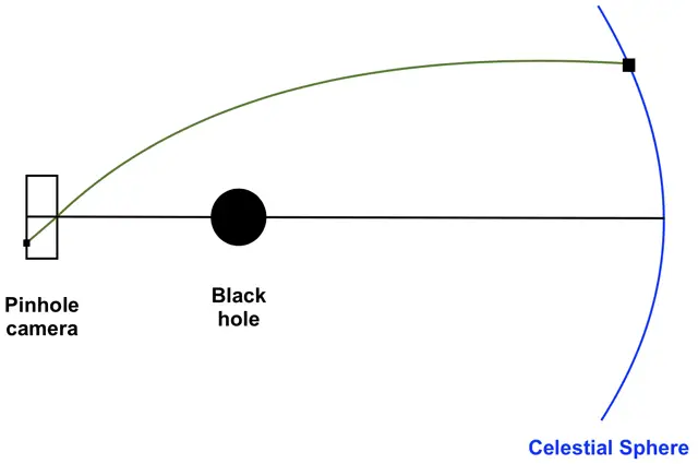
To produce images of Schwarzschild black holes our code will need to ray trace the photons paths. The images will be what appears from a camera that is looking directly at a black hole with a celestial sphere star field at an infinite distance behind it. This is shown in Figure 3.1 where a pinhole camera is on the left, the black hole is the black disc in the centre and a star field on a celestial sphere is on the right. In this figure we see a photon path, the green line, starting from a point on the celestial sphere being diverted around the black hole and still ending in the pinhole camera. So from the pinhole camera’s perspective the image of the point on the celestial sphere looks like it is coming from a different direction than it actually is.
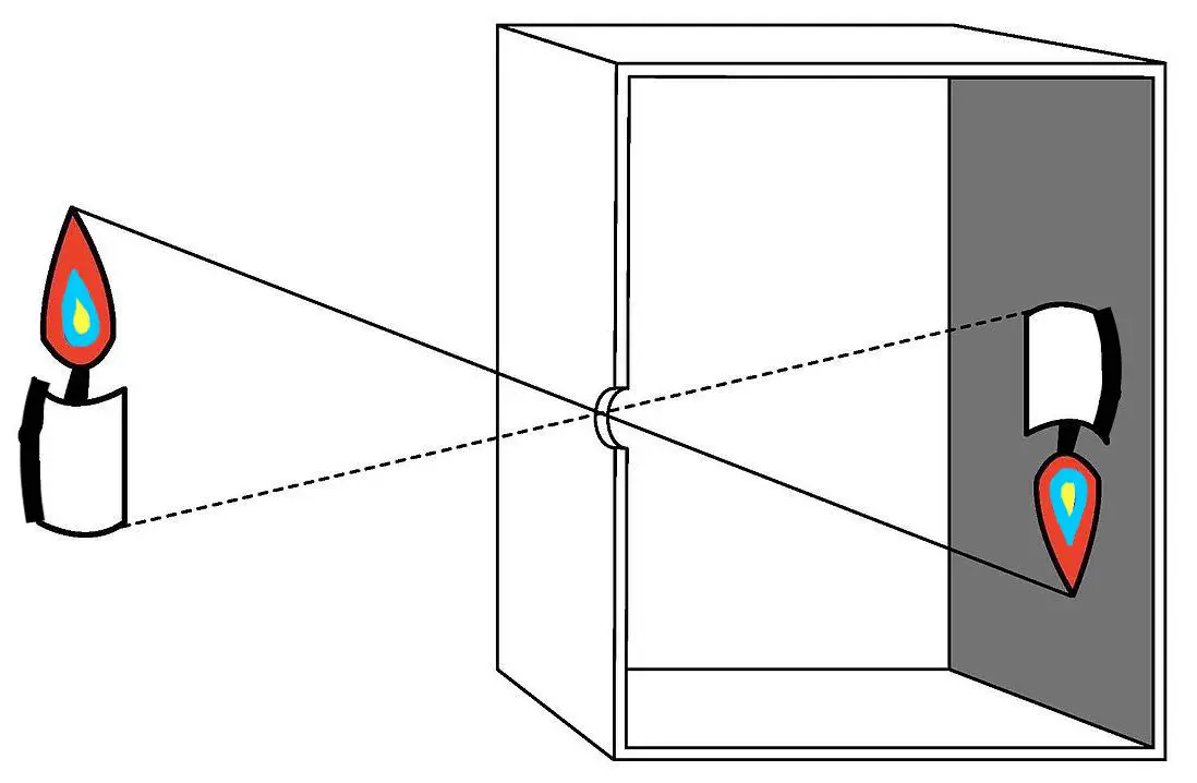
Pinhole cameras work by having an infinitesimally small hole in a
light-proof box as shown in Figure 3.2. When light from
various angles pass through this aperture it forms an image that has
been inverted both vertically and horizontally on a photographic plate
on the opposite side of the box. The width of the lightproof box is
known as it focal length,
,
which is a constant we set before running the code. The focal length
affects how much light passes into the box, to determine the size and
view of the image. The code produces the images by modelling what
appears on the photographic plate of a pinhole camera in Figure 3.2.
To ray trace these paths an integrating function in python solves the three first order differential equations for the Schwarzschild Geometry, by starting the photons at the aperture of the pinhole camera and iterates over each time step, by integrating the equations to produce an array, (), of the photon’s location at each time step. This function uses the initial values of () are used to find solutions of the derivatives for each time step.It then integrates over the functions to produce the array of the photon’s locations as for each time step from to . Setting the amount of time steps to a very large integer, gives an accurate location of the photon’s location when . Plotting the array of locations of the photon shows the paths that the light travels along in two dimensions around and near the black hole. Using a range of values of angular momentum, , for the photons we see the different paths that light travels along.
t  = np.linspace(0,1000,200) # time steps
yo = [2, 3]                  # constants [M, L]
zo = [np.pi, 20, -0.13]      # initial [phi0, r0, s0]

def function(z, t, y):      # ODE functions
    phi, r, s = z
    M, L = y

    dpdt = L/r**2
    drdt = s
    dsdt = -(L**2)*(3.0*M-r)/(r**4)
    return [dpdt, drdt, dsdt]

z = scipy.integrate.odeint(function,zo,t, args=(yo,))  # solve ODE
phi, r, s = z[:,0], z[:,1], z[:,2]
Ray tracing these light paths for each pixel on the photographic plate will take the code large periods of time to run and produce good quality images, so it would be an ineffective method. To speed up the code, we find a relation between the curvature of the light paths, which generalises for all paths near the black hole. Because this is a symmetric problem we can find a correlation between two different angles in the two dimensional plane. Figure 3.3 shows the first angle being , which is the angle under which a star’s light would classically enter the camera’s aperture in the absence of the black hole, which is the star’s natural angle as it would be in Newtonian physics. The second angle, , in Figure 3.3 is the angle at which the light from the same star actually enters the camera’s aperture due to the bending caused by the black hole’s gravitational field. Both of these angles will be measured with respect to the horizontal in the black hole’s equatorial plane.
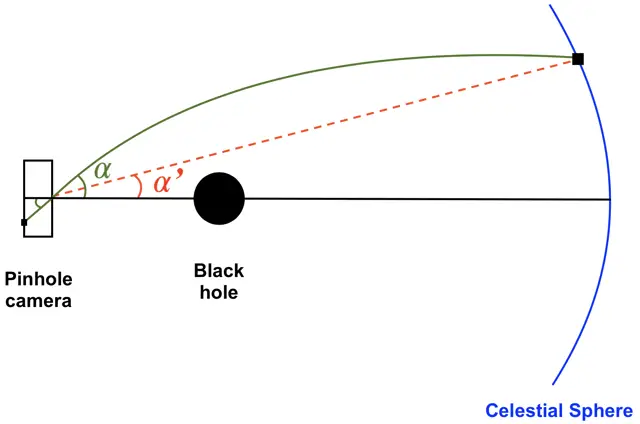
These angles are calculated simply by comparing the different locations of photons and using their change in positions. To get the real angle of the star, , the end location of the photon is recorded after many time iterations to get the angle which is what tends to when you hit the celestial sphere because it is at an infinite distance away. The angle is calculated using trigonometric equations using the change in location of the photon between the first two time steps. After getting a list of various angles of and by using many different values of angular momentum, , an interpolating function in python produces a map from by comparing the relations in values of the two angles. This map acts as a function that after an angle is entered into it, it finds the corresponding value of .
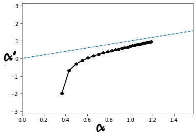
This map between and has been plotted, shown in Figure 3.4, where as you would expect for small angles of the plot has no corresponding values as the photons have been absorbed by the black hole and cannot escape. For this reason there do not exist any values lower than this one, as there are limitations to the amount of gravitational lensing that can occur. This is when light travels around the black hole in different directions and intersect in the future, which will be explained in more detail in the next chapter. The photon that has the maximum curvature around the black hole is plotted with the smallest value of , hence no plots exists below this. Increasing from this point the plot is steep with a large gradient and corresponds to negative values, which has been caused by photons traveling from the lower side of the celestial sphere, curving up and around the top of black hole and still making it to the pinhole camera. As gets larger, and closer to , the graph becomes less steep and the values of and tend to , represented by the straight blue dashed line. This occurs because when the photons are traveling further away from the black hole, they are less curved by it, causing the map of the angles to have a direct correlation. For negative values the plot would appear as the plot in Figure 3.4 reflected in the line.
Another angle, , is introduced to generalise, by rotational symmetry, our model to a three dimensional problem as was removed from the line metric equation to simplify the ray tracing in the two dimensional equatorial plane. The angle will be defined as the angle between the photon and the direct vertical, which we were using as the equatorial plane. In this model light paths will only be traced in two dimensions, so that the angle will not be affected by the curvature of spacetime. The only change to will be from the pinhole camera. So after the photon has left the pinhole camera, the angle is just inverted horizontally and vertically as we pass the black hole because the Schwarzschild geometry is symmetric and because of the properties of pinhole cameras. So this relation is defined as .
Now that all of the crucial steps of ray tracing have been covered, a backwards ray tracing algorithm can now be derived to produce the black hole images.
3.4 The Backwards Ray Tracing Algorithm
To produce these images of Schwarzschild black holes, a code with an algorithm that will be outlined below is used. The following steps need to be taken for the code to produce an image of a black hole:
Set the initial location of the pinhole camera’s aperture, at , the focal length, , and the mass of the black hole, .
Start at a pixel, , on the photographic plate of the pinhole camera and calculate the angles and of this photon. This is done by using the change in distances of this pixel from the centre of the photographic plate as shown in the left image of Figure 3.5. It is showing the photographic plate of width and height in pixels, the change in vertical and horizontal distance, , and the hypotenuse of the triangle being . These equations are defined as follows:
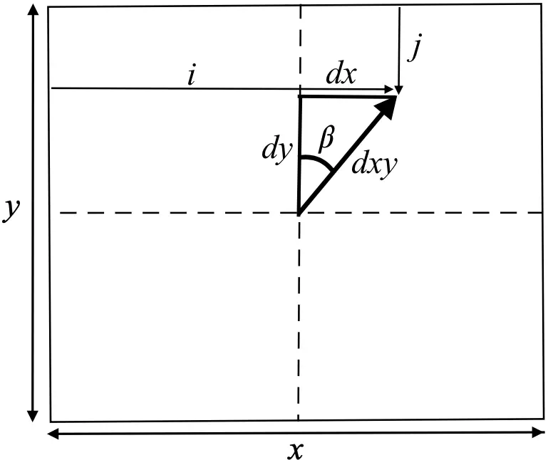
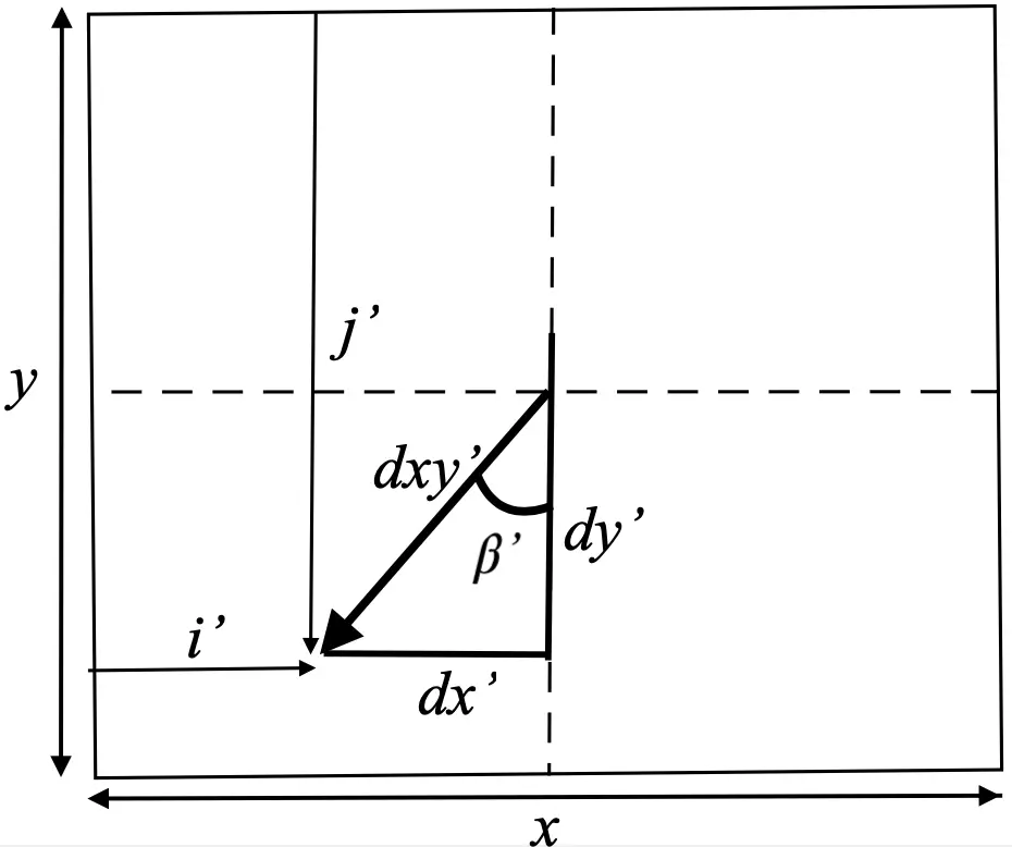
Figure 3.5: The figure on the left is the photographic plate, with dimensions by , of the pinhole camera, showing the angle of pixel , and the change in height, , and width, , of this pixel from the centre of the image. The figure on the right is similar, except it is the image of the flat celestial sphere that is attached in our code, with new pixel coordinates, , and angle . The angle is calculated using the focal length, , and the distance of the photon from the centre of the photographic plate as
The angle is calculated by using the position of the pixel compared to the vertical, which changes depending on which side of the photographic plate it is on. This angle is defined by
The interpolating function discussed in the previous section is used to map , . This gives when is larger than the greatest value in the plot in Figure 3.4 because the plot tends towards the blue dashed line. For the rest of the values, the interpolating map is used to evaluate . The angle is just inverted horizontally and vertically as we pass the black hole so therefore we get .
Use to calculate the location of where the photon would have originally come from on the celestial sphere. Calculate this pixel on the celestial sphere, , by first calculating the change in distances on the celestial sphere image on the right image of Figure 3.5, with
The red, green and blue colour scheme is used where each pixel on the celestial sphere is assigned three integer values between and depending on its colour. Then, the colour of the pixel, , is extracted from the celestial sphere, so that the corresponding pixel, , on the photographic plate takes this colour.
If the photon from a pixel does not make it to the celestial sphere and is instead absorbed by the black hole you set the colour of that pixel as (0,0,0), which represents the colour black, as no light has been absorbed from this direction. This is if the angle of is lower than that of the lowest point plotted in our Figure 3.4.
Repeating this for all pixels, for , , on the photographic plate produces a deformed image of a Schwarzschild black hole.
Now that the photon’s equations of motions in the Schwarzschild geometry have been derived and used in our piece of code that contains the algorithm to ray trace and produce images of these black holes, we can move onto analysing the images of the black holes.