Chapter 2: General Relativity and Tensor Calculus

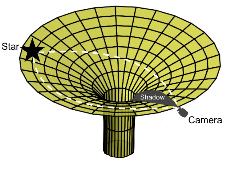
In 1915 Albert Einstein developed a theory that massive objects like black holes generate a strong gravitational field that causes the warping of the spacetime geometry around it, which is known as general relativity. In Figure 2.1, a black hole, represented at the bottom of the tunnel, has caused the spacetime around it to curve. As a result of this, paths of photons from the star curve along the manifold’s surface, whereas classically in Newtonian physics the light rays from the star would travel along straight lines to the camera. The angle under which the camera now sees the star is different from the actual angle the star is at, making the star appear to be at a different location than it actually is. To express this curvature in numerical form the following concepts of tensor calculus will be used to describe different spacetime geometries. Most of the work in this chapter has come from Shultz’s book ^[1] and Hobson’s book ^[2]. Where other books are used, they will be stated.
To express this bending of objects around black holes we will first need to consider how the distances between events in on a curved spacetime can be expressed numerically.

2.1 Line Elements and the Metric Tensor

To find equations explaining the distance between events on curved manifolds, the distances between extremely near points are measured as the manifold tends towards a flat surface when we consider an infinitesimally small area on it. This work is based on work by Shultz’s book ^[1] in Chapter 3.

If there exists an infinitesimally small distance, $dx^\alpha$, between two points $A$ and $B$, with coordinates $x^\alpha$ and $x^\alpha +dx^\alpha$ respectively, then the separation of $AB$ is a vector defined as $d\vec{s} = dx^\alpha \vec{e_\alpha}$. The length of this vector then becomes $$\begin{aligned} ds^2 &= (dx^\alpha \vec{e_\alpha}) \cdot (dx^\beta \vec{e_\beta})= (\vec{e_\alpha} \cdot \vec{e_\beta}) dx^\alpha dx^\beta. \\ \end{aligned} \label{a1}$$ The scalar product of the basis vectors can then be defined as a matrix $g_{\alpha\beta}$ with $\alpha$ rows and $\beta$ columns, shown by $$\begin{aligned} (\vec{e_\alpha} \cdot \vec{e_\beta}) &= g_{\alpha\beta}.\\ \end{aligned} \label{a2}$$ Replacing this matrix notation into our equation gets $$ds^2 = g_{\alpha\beta}(x) dx^\alpha dx^\beta. \label{1}$$ This equation contains the distance between all points in space. To generalise this to objects in different kinds of spacetime, a comparison between different types of distance intervals needs to be introduced and an understanding of how objects move along in different spacetimes is needed.

A world line of an object is the positions in space that the object can be located at different times. Along these world lines the time an object experiences is known as the object’s proper time, $\tau$. This can be understood more clearly by saying it is the time on a clock that is moving along with that object. This is because in special relativity when objects move at fast speeds similar to that of the speed of light, an object’s real time, $\tau$, changes relative to other objects that are not moving. For this reason we have three different types of distance intervals in space time:

• The first being when $ds^2 > 0$, when the object has a time-like interval, which means an inertial frame can be found where events can happen at the same spatial coordinates.

• The second when $ds^2 = 0$, it is light-like or null separated, this is when massless particles such as photons travelling at the speed of light, $c$, are considered to have no real time between events in spacetime. This is the distance interval we will be using most in this report as we study how light rays in the form of photons affect the appearance of black holes.

• The third when $ds^2 < 0$, it is space-like, which means that an inertial frame can be found that can have events occurring at the same time coordinate.

Now that distance intervals have been defined, line metrics and metric tensors can be explained in spacetime.

The equation above is known as a line metric, which is used to describe how space changes at a point on a curved spacetime surface. It encodes the distance between points in spacetime. The $g_{\alpha\beta}$ element represents a metric tensor, which is a matrix that corresponds to the elements used to calculate small distances between changing coordinates at a point in spacetime.

The metric tensor matrix is shown as $$g_{\alpha,\beta} = \begin{pmatrix} a_{1,1} & a_{1,2} & \cdots & a_{1,n} \\ a_{2,1} & a_{2,2} & \cdots & a_{2,n} \\ \vdots & \vdots & \ddots & \vdots \\ a_{m,1} & a_{m,2} & \cdots & a_{m,n} \end{pmatrix}. \label{mat2}$$ The difference in coordinates between points is multiplied by the corresponding $\alpha, \beta$ element of the matrix. When these are summed over all possible combinations, the equation takes the same form as the line element:

$$ds^2 = g_{\alpha\beta}(x) dx^\alpha dx^\beta. \label{eq1}$$

Line metrics will be used as a coordinate system that describes the position of objects in spacetime. Multiple different coordinate systems can be used to describe the same spacetime. We will now discuss how both Cartesian and polar coordinates can be used in the Minkowski spacetime.

2.2 Euclidean Geometries and the Minkowski Spacetime

In a Minkowski spacetime, $\eta_{\alpha\beta}$, with Cartesian coordinates $x^\alpha = (t, x, y, z)$, the metric tensor matrix, equation matrix below, only has orthogonal $1$’s, and a $-1$ in the double time component, with zeros everywhere else. The cross product of the derivative of two different coordinates are equal to zero, because the coordinates are perpendicular to each other. These are shown in the below equations as:

$$\begin{aligned} \vec{e_i} \cdot \vec{e_i} &= 1 , \text{ for } i \in (x,y,z),\\ \vec{e_t} \cdot \vec{e_t} &= -1,\\ \vec{e_i} \cdot \vec{e_j} & = 0 \text{ for } i,j \in (t,x,y,z) \text{ with } i \neq j .\\ \end{aligned} \label{3}$$ The negative $-dt^2$ means that $ds^2$ goes up in a time-like direction and because there is no constant multiplied to it, it is measured in the objects proper time, $\tau$, at rest in space. The completed metric tensor of Cartesian coordinates in the Minkowski spacetime becomes

$$\eta_{\alpha,\beta} = \begin{pmatrix} -1 &0 & 0 & 0 \\ 0 & 1 & 0& 0\\ 0 & 0 & 1&0 \\ 0& 0 & 0 & 1 \end{pmatrix}. \label{4}$$ The line metric for this space time in these coordinates is therefore $$\begin{aligned} ds^2 &=\eta_{\alpha\beta}dx^\alpha dx^\beta = -dt^2 + dx^2 +dy^2 + dz^2.\\ \end{aligned} \label{eq5}$$

The line metric for spherical coordinates, $(t, r, \theta, \phi)$, in Minkowski spacetime are derived below, by turning Cartesian into spherical coordinates. This spherical coordinate system will be used throughout the report because the Schwarzschild black holes and the wormholes we will be modelling are symmetric. With $x,y \text{ and } z$ being defined in the usual way with $$\begin{aligned} x &= r\sin{\theta} \cos{\phi},\quad y = r\sin{\theta} \sin{\phi} , \quad z = r\cos{\theta}.\\ \end{aligned} \label{6}$$ Working out their derivatives, $dx, dy, dz$ as

$$\begin{aligned} dx &= dr\sin{\theta} \cos{\phi} + r\cos\theta \cos\phi d\theta- r\sin (\theta)\sin\phi d\phi,\\ dy &= dr \sin{\theta} \sin{\phi} + r \sin{\phi} \cos\theta d\theta + r\sin\theta \cos\phi d\phi,\\ dz &= dr \cos\theta - r \sin\theta d\theta.\\ \end{aligned} \label{7}$$ Squaring the derivative components above and then substituting them into the line metric equation for space-time in these coordinates gives

$$\begin{aligned} ds^2 &=g_{\alpha\beta}dx^\alpha dx^\beta = -dt^2 + dr^2 + r^2(d\theta^2 + \sin ^2 \theta d \phi^2).\\ \end{aligned} \label{8}$$ With the metric tensor matrix in spherical coordinates being $$g_{\alpha,\beta} = \begin{pmatrix} -1& 0 & 0 & 0 \\ 0 & 1 & 0 & 0 \\ 0 & 0 & r^2& 0 \\ 0 & 0 & 0 & r^2\sin^2\theta\\ \end{pmatrix}. \label{9}$$ Now that the distance between two events in spacetime has been derived to produce a line metric, we need to find equations that govern the paths that objects in spacetime move along.

2.3 Deriving the Geodesic Equations

To model the geometry of an object’s world line, a set of equations need to be derived, to connect different locations of objects along them. This derivation is from work by Hartle, ^[3], in Chapter 8.1. The proper time from a point $A$ to a point $B$ on the world line of a time-like object is calculated by integrating the square root of its line metric along the world-line as

$$\begin{aligned} \tau_{AB} &= \int_{A}^B d\tau = \int_{A}^B (-g_{\alpha\beta}(x) dx^\alpha dx^\beta)^\frac{1}{2}.\\ \end{aligned} \label{10}$$ By introducing a parameter, $\sigma$, that the world line depends upon, with $\sigma$ ranging from 0 at point $A$ to 1 at point $B$, causes the equation to become $$\begin{aligned} \tau_{AB} &= \int_{0}^1 d\sigma \left(-g_{\alpha\beta}(x) \frac{dx^\alpha}{d\sigma} \frac{dx^\beta}{d\sigma}\right)^\frac{1}{2}.\\ \end{aligned}$$ Rearranging to give an expression of $\frac{d\tau}{d\sigma}$ which will be used to substitute in later as $$\begin{aligned} \frac{d\tau}{d\sigma} &= \left(-g_{\alpha\beta}(x) \frac{dx^\alpha}{d\sigma} \frac{dx^\beta}{d\sigma}\right)^\frac{1}{2}.\\ \end{aligned}$$ To maximise this proper time, $\tau$, along the world line a solution to the Lagrange equation needs to be found. With the Lagrange equation as $$\begin{aligned} -\frac{d}{d\sigma}\left(\frac{\partial L }{\partial(dx^\alpha/d\sigma)}\right) +\frac{\partial L }{\partial x^\alpha} &= 0,\\ \end{aligned} \label{.3}$$ with the Lagrangian set as $$\begin{aligned} L \left(\frac{dx^\alpha}{d\sigma},x^\alpha\right) &= \left(-g_{\alpha\beta}(x) \frac{dx^\alpha}{d\sigma} \frac{dx^\beta}{d\sigma}\right)^\frac{1}{2}.\\ \end{aligned} \label{.2}$$

Substituting the Lagrangian equation into equation above it gives $$\begin{aligned} -\frac{d}{d\sigma}\left( \left( -g_{\zeta\eta}(x) \frac{dx^\zeta}{d\sigma} \frac{dx^\eta}{d\sigma}\right)^{-\frac{1}{2}} \left( g_{\alpha\beta}(x) \frac{dx^\beta}{d\sigma}\right)\right) +\frac{1}{2}\left( -g_{\zeta\eta} \frac{dx^\zeta}{d\sigma} \frac{dx^\eta}{d\sigma}\right)^{-\frac{1}{2}} \frac{\partial g_{\epsilon\beta} }{\partial x^\alpha}\frac{dx^\epsilon}{d\sigma} \frac{dx^\beta}{d\sigma} &= 0,\\ -\frac{d}{d\tau}\left( \left( g_{\alpha\beta}(x) \frac{dx^\beta}{d\tau}\right)\right) +\frac{1}{2}\frac{\partial g_{\beta\zeta} }{\partial x^\alpha}\frac{dx^\beta}{d\tau} \frac{dx^\zeta}{d\tau} &= 0,\\ -\frac{dg_{\alpha\beta}}{d\tau}\left( \frac{dx^\beta}{d\tau}\right) -dg_{\alpha\beta}\frac{d^2x^\beta}{d\tau^2}+\frac{1}{2}\frac{\partial g_{\beta\zeta} }{\partial x^\alpha}\frac{dx^\beta}{d\tau} \frac{dx^\zeta}{d\tau} &= 0\\ \end{aligned} \label{.4}$$ To simplify the equation’s expressions, $\partial_{\gamma}g_{\alpha\beta}$ is used as the shortened notation of the partial derivative of our metric matrix with indices $\alpha,\beta$ with respect to $x^\gamma$ as $\left( \partial_{\gamma}g_{\alpha \beta} = \frac{\partial g_{\alpha \beta}}{ \partial x^{\gamma}}\right)$. Rearranging the last expression in this equation, simplifying the dummy indices and then multiplying both sides by the inverse of our metric tensor, $g^{\alpha \beta}$, with indices $\alpha \beta$, then gives

$$\begin{aligned} g_{\alpha\beta}\frac{d^2x^\beta}{d\tau^2} &= \left(-\frac{\partial g_{\alpha\beta} }{\partial x^\zeta} +\frac{1}{2}\frac{\partial g_{\beta\zeta} }{\partial x^\alpha}\right) \frac{dx^\beta}{d\tau} \frac{dx^\zeta}{d\tau}, \\ g_{\alpha\eta} \frac{d^2x^\eta}{d\tau^2} &= -\frac{1}{2} \left(\partial_{\zeta}g_{\alpha\beta}+ \partial_{\beta}g_{\alpha\zeta}- \partial_{\alpha}g_{\beta\zeta}\right)\frac{dx^\beta}{d\tau} \frac{dx^\zeta}{d\tau},\\ \frac{d^2x^\eta}{d\tau^2} &= -\frac{1}{2} g^{\eta\alpha} \left(\partial_{\zeta}g_{\alpha\beta}+ \partial_{\beta}g_{\alpha\zeta}- \partial_{\alpha}g_{\beta\zeta}\right)\frac{dx^\beta}{d\tau} \frac{dx^\zeta}{d\tau}.\\ \end{aligned} \label{13}$$ This equation can be simplified further by defining Christofell symbols, which contain information of how an object’s space time grid is changing, locally, in each direction. It is defined as $$\begin{aligned} \Gamma^{\eta}_{\beta\zeta} &= \frac{1}{2} g^{\eta\alpha} (\partial_{\zeta}g_{\alpha\beta}+ \partial_{\beta}g_{\alpha\zeta}- \partial_{\alpha}g_{\beta\zeta}).\\ \end{aligned} \label{14}$$ Substituting the Christofell symbol into the last expression of the equation above it gives $$\frac{d^2 x^\eta}{d\tau^2} = -\Gamma^{\eta}_{\beta\zeta}\frac{dx^\beta}{d\tau} \frac{dx^\zeta}{d\tau}.\\ \label{15}$$ These equations are known as the Geodesic equations. A geodesic is a straight line in Euclidean space, that is the shortest distance between two points in spacetime. Along each geodesic there exists a vector that is tangent to this line, always pointing in the same direction. This equation predicts the trajectories of objects in space time.

The geodesic equations above were derived around free particle paths with time-like distance intervals. This cannot be used for the null world lines of light paths with light-like intervals. Instead a new affine parameter $\lambda$ (which does not affect the geodesic equations) is introduced that light-like objects depend on. This is because light travels no real distance in spacetime, $ds^2 = 0$, so it cannot depend on its real time as it does experience time when it travels at the speed of light. The trajectories of light rays cannot be traced by just equating its line metric to zero, instead the geodesic equation is no longer parametrised by the proper time, $\tau$, of the light ray but rather by the parameter $\lambda$, which equates the null geodesics as

$$\frac{d^2 x^\alpha}{d\lambda^2} = -\Gamma^{\alpha}_{\beta\gamma} \frac{d x^\beta}{d\lambda} \frac{d x^\gamma}{d\lambda}.\\$$

These time-like geodesics are going to be used in the following chapters as light is traced around black holes and wormholes. To calculate equations of motions of particles along these geodesics we need to learn the tensor calculus necessary to find them.

2.4 The Curvature Tensor

To numerically describe the curvature of a manifold in spacetime, a curvature tensor is introduced. Information in the following chapter was based on the work of Hobson, ^[2], in Chapter 7.9-7.11.

To express this curvature numerically, we need to compare the results of changing the order of the covariant derivative, $\Delta_\alpha$, acting on a manifold’s vector field. A covariant derivative acts in the same way as partial derivatives do, except that changing the order of the derivatives acting on a term does change the final result. Taking this covariant derivative with respect $b$ on a vector $v_a$ gives

$$\begin{aligned} \Delta_b v_a &= \partial_b v_a -\Gamma^{d}_{ab} v_d. \\ \end{aligned} \label{19b}$$ Adding an additional covariant derivative with respect to a different coordinate, $c$, gives $$\begin{aligned} \Delta_c \Delta_b v_a &= \partial_c (\Delta_b v_a ) -\Gamma^{e}_{ac} \Delta_b v_e -\Gamma^{e}_{bc} \Delta_e v_a,\\ &=\partial_c \partial_b v_a - (\partial_c \Gamma^{d}_{ab}) v_d - \Gamma^{d}_{ab}\partial_c v_d -\Gamma^{e}_{ac} (\partial_b v_e -\Gamma^{d}_{eb}v_d) -\Gamma^{e}_{bc} (\partial_e v_a -\Gamma^{d}_{ea}v_d) .\\ \end{aligned} \label{20}$$ Taking the difference of this equation with the term where the covariant derivatives acted in a different order $(\Delta_b \Delta_c v_a)$ becomes $$\begin{aligned} \Delta_c \Delta_b v_a - \Delta_b \Delta_c v_a &= R^d_{abc} v_d.\\ \end{aligned} \label{21}$$ So the difference of these two terms gives us the curvature tensor, $R^d_{abc}$, defined as $$\begin{aligned} R^d_{abc} &\equiv \partial_b \Gamma^{d}_{ac} -\partial_c \Gamma^{d}_{ab} + \Gamma^{e}_{ac} \Gamma^{d}_{eb} - \Gamma^{e}_{ab} \Gamma^{d}_{ec} .\\ \end{aligned} \label{22}$$ The Riemann tensor or curvature tensor fully describes the geometry of a manifold in all directions. In a four dimensional spacetime there are $256$ elements of this curvature tensor. When the curvature tensor vanishes at every point on a manifold, as in equation below, then the manifold is flat, which is why the flat Euclidean plane of the Minkowski geometry has their curvature tensor as

$$R^d_{abc} = 0 . \\ \label{25}$$ This Riemann tensor contains many symmetries. After expressing it in terms of the metric tensor, $R_{abcd} = g_{ae}R^e_{bcd}$, and expanding the terms in it, the following symmetries appear: $$\begin{aligned} R_{abcd} &= -R_{bacd}, \\ R_{abcd} &= -R_{abdc}, \\ R_{abcd} &= R_{cdab}. \\ \end{aligned} \label{26a}$$ The multiple symmetries in these equations above can be simplified into an easier tensor, which can be defined when the first and fourth indices are equal on the curvature tensor. This is known as the Ricci tensor which is defined as $$R_{ab} \equiv R^c_{abc}. \\ % R_{ab} \equiv R^c_{abc} = R^c_{bac} = R_{ba}\\ \label{26}$$ The curvature scaler or Ricci scalar is a value corresponding to the average curvature in all directions at each point on a manifold. Defined as $$R \equiv g^{ab} R_{ab}= R^a_a. \\ \label{26b}$$ Following on from when the Riemann tensor is equal to zero, as expected the Ricci scalar in Euclidean space is zero as it is a flat manifold. Now that the curvature of a manifold can be expressed numerically, we will now start looking at tensors that are related to the energy and momentum of objects in spacetime.

2.5 Einstein Tensor and the Energy Momentum Tensor

Two new tensors are introduced in this section using the work of Hobson, ^[2], Chapters 7.11 and 8.

After taking the covariant derivative of the Ricci tensor and Ricci scalar, from equations above, an important relation appears. This relation is $$\begin{aligned} \Delta_b \left(R^{bc} - \frac{1}{2}g^{bc} R\right) &=0 .\\ \end{aligned} \label{30}$$ We define this term in parentheses as the Einstein tensor with $$\begin{aligned} G^{ab} &\equiv R^{ab} - \frac{1}{2}g^{ab} R = G^{ba}.\\ \end{aligned} \label{31}$$ The Einstein tensor is clearly symmetric because of the properties of the Ricci tensor and metric tensor, hence this tensor also describes the curvature of spacetime.

A tensor needs to be introduced to contain information about the matter distribution at each event in a spacetime. The energy momentum tensor is then defined as $$\begin{aligned} T(x) & = \rho_0(x) u(x) \otimes u(x) \\ \end{aligned} \label{32}$$ with $\rho(x)$ being the fluid’s proper density, that is measured by an observer moving along the same world line. The $u(x)$ element is the object’s $4$ velocity, which can be generalised to a $x^\alpha$ coordinate system to give the energy momentum tensor as $$\begin{aligned} T^{\alpha \beta} & = \rho u^\alpha u^ \beta. \\ \end{aligned} \label{33}$$

After lengthy equations of fluid mechanics, using relativistic continuity equations, as shown in Hobson’s work, ^[2], Chapter 8.3, we arrive at a result about the conservation of energy momentum for a perfect fluid, with $$\begin{aligned} \Delta_\alpha T^{\alpha \beta} & = 0. \\ \end{aligned} \label{34}$$ Combining these two special relations, an important equation emerges that is some of Einstein’s best work, which relates the matter in a spacetime to it’s geometry.

2.6 The Einstein Field Equations

Work from this section has been derived from the work of Hobson, , Chapter 8.4. Combining the equations from the previous section together, and adding a potential constant, $\kappa$, gives $$\begin{aligned} R^{\alpha\beta} - \frac{1}{2}g^{\alpha\beta}R &= -\kappa T^{\alpha\beta}. \\ \end{aligned} \label{35}$$ To find the value of $\kappa$ observations and known results of a weak static gravitational field in the low velocity limits are combined to give $$\begin{aligned} \vec{\Delta}^2 g^{00}R & = \frac{8\pi G}{c^4} T^{00}. \\ \end{aligned} \label{36}$$ Hence the value $\kappa = \frac{8\pi G}{c^4} = 8\pi$ is derived to give the Einstein’s gravitational field equations as

$$\begin{aligned} R^{\alpha\beta} - \frac{1}{2}g^{\alpha\beta}R & = 8\pi T^{\alpha\beta}. \\ \end{aligned} \label{37}$$ These field equations relate the distribution of matter and energy on a spacetime with the geometry’s curvature at each point on it. The unique solution of these equations are used to calculate the line metrics of different spacetime geometries. This is a tedious process because the tensors contain multiple elements and hence multiple equations need to be solved in order to find the metrics.

Now that we have covered enough general relativity to understand the tensor calculus behind Einstein’s equations and have the knowledge of how to derive line metrics in spacetime, we will start looking at our first black hole geometry known as the Schwarzschild geometry.